I chose to implement texture mapping on spheres and triangles for all components of the lighting model. This meant that the following parameters could each be specified by unique texture maps: diffuse color, specular color, ambient color, shininess (size of the Phong highlight), surface normal (bump map), and "roughness" (see section 2 for more details). I had removed transparency from my lighting model for homework 2 and did not re-implement it for homework 3. Thus, transparency is not one of the parameters that can be texture mapped. It could easily be added to the texture mapping algorithm, however.
The ".out" scene format output by "composer" specifies texture coordinates for triangles. However, it does not provide support for specifying a file from which to read a texture. Nor does it provide texture orientation (axis and meridian) for spheres. Additionally, information about which texture to apply to which part of the lighting model is not supplied. I had to specify this information in a separate "map" file. For any scene file "scene.out" or "scene.ascii", I read in an ASCII file "scene.map" containing texture information. The "scene.out" scene format provides for a name for each object, so I used that name to apply information to the object. These names are referred to in my the file. An example of such a file is:
sphere diffuse globe axis 0;1;0 meridian 1;0;0
ground diffuse wood bump bumpiness roughness checker
- diffuse
- specifies a texture for the diffuse color map.
- specular
- ambient
- specifies a texture for the ambient color map.
- shininess
- specifies a texture map for the "shininess", the size of the Phong reflection. Only the red component of the texture map is used. High values correspond to high exponents. Low values correspond to low exponents.
- roughness
- specifies a texture map for the "roughness", or degree of diffuse reflection. More on this in section 2, below.
- bump
- specifies a texture map for the surface normal. The texture map is used to modify the original surface normal. The red component of the texture map is used to deflect the normal in the "X" direction and the green component of the texture map is used to deflect the normal in the "Y" direction. More on this below.
- axis
- A semicolon-delimited vector specifying the "up" direction for spheres. This defines the starting point of the t parameter of the texture coordinates.
- meridian
- A semicolon-delimited vector specifying the "meridian" direction for spheres. This defines the starting point of the s parameter of the texture coordinates.
-
specifies a texture for the specular color map. Note that the color also
defines the degree of reflectivity of the surface. White points are highly
reflective, grey points are halfway reflective, and black points are least
reflective.
To specify the correspondence between texture names and PPM image files, a global "texture" file is read in. This ASCII file is located in the current working directory. Each line of the file has a texture name, a space, then the absolute path name of a PPM image file to be used for that texture.
At each point on a surface, texture coordinates are generated.
 For spheres, this is done by using some dot products and arccosines.
(Expensive, I know, but I haven't yet come up with a better way of doing
it.) The point on the surface P is turned into a
vector from the origin of the sphere. The angle phi
between P and the axis is found using a dot product
and an arccosine. This angle can vary between 0 and 180 degrees. This is
scaled to be between 0.0 and 1.0 for the t texture coordinate. Then the
P vector is projected onto the equator of the
sphere. The angle theta between the projected
vector and the meridian is found again using a dot product and an arccosine.
This angle can vary between 0 and 180. To handle textures on the opposite side
of the sphere, a cross product is taken to determine which side of the sphere
the vector P lies on. Based on theta and the result of the cross product, a texture
coordinate s is created that varies between 0.0 and 1.0.
For spheres, this is done by using some dot products and arccosines.
(Expensive, I know, but I haven't yet come up with a better way of doing
it.) The point on the surface P is turned into a
vector from the origin of the sphere. The angle phi
between P and the axis is found using a dot product
and an arccosine. This angle can vary between 0 and 180 degrees. This is
scaled to be between 0.0 and 1.0 for the t texture coordinate. Then the
P vector is projected onto the equator of the
sphere. The angle theta between the projected
vector and the meridian is found again using a dot product and an arccosine.
This angle can vary between 0 and 180. To handle textures on the opposite side
of the sphere, a cross product is taken to determine which side of the sphere
the vector P lies on. Based on theta and the result of the cross product, a texture
coordinate s is created that varies between 0.0 and 1.0.
For triangles, the texture coordinates are generated by doing a bi-linear interpolation of the texture coordinates at the vertices.
For simplicity, no correction is done for perspective. In my sample renderings, this doesn't seem to significantly impact the results.
Once texture coordinates are generated, the material for the surface may be generated. The global material for the surface is used as a starting point. Then, for each component that is specified as being texture mapped, an image lookup is done using the texture coordinates. No interpolation of the pixel values is done; only the pixel found is returned. In this way, a new material is calculated for each intersection point, and shading calculations are done on this calculated material.
 In addition to the material, the surface normal may be generated if bump
mapping is specified. This is done by first determining the actual surface
normal N. Then an orthogonal coordinate system is generated with N, the
original surface normal, used as one of the axis. The other two axes are S =
[1 0 0] x N and T = S x N. The red component of the texture map (scaled from
0.0 to 1.0) is used to scale the S axis, and the green component (scaled from
0.0 to 1.0) is used to scale the T axis. Thus, the resultant normal vector is
found V = N + s*S + t*T. (Note that the choice of [1 0 0] to construct the
coordinate system can cause problems when the surface normal crosses the world
X axis ([1 0 0]). A more intelligent way of generating the coordinate system
would provide better results.)
In addition to the material, the surface normal may be generated if bump
mapping is specified. This is done by first determining the actual surface
normal N. Then an orthogonal coordinate system is generated with N, the
original surface normal, used as one of the axis. The other two axes are S =
[1 0 0] x N and T = S x N. The red component of the texture map (scaled from
0.0 to 1.0) is used to scale the S axis, and the green component (scaled from
0.0 to 1.0) is used to scale the T axis. Thus, the resultant normal vector is
found V = N + s*S + t*T. (Note that the choice of [1 0 0] to construct the
coordinate system can cause problems when the surface normal crosses the world
X axis ([1 0 0]). A more intelligent way of generating the coordinate system
would provide better results.)
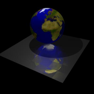
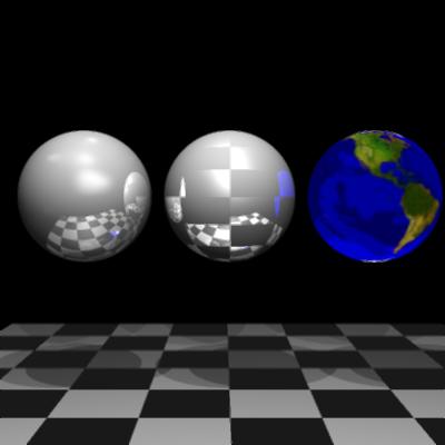 The image on the right (click for a larger version), of three spheres and a
ground plane, illustrates diffuse mapping, specular mapping, shininess mapping,
and ambient mapping. The ground plane is diffuse mapped with a checker pattern
of alternating white and black squares. The sphere on the left has the same
image used as its shininess map. Note that the size of the four Phong
highlights change across the surface of the sphere. The sphere in the middle
uses the checker image again for its specular map. Since black means to have
no reflection and white means perfect reflection, the sphere alternates
reflection across its surface. The sphere on the right uses a map of the Earth
as its ambient texture map.
The image on the right (click for a larger version), of three spheres and a
ground plane, illustrates diffuse mapping, specular mapping, shininess mapping,
and ambient mapping. The ground plane is diffuse mapped with a checker pattern
of alternating white and black squares. The sphere on the left has the same
image used as its shininess map. Note that the size of the four Phong
highlights change across the surface of the sphere. The sphere in the middle
uses the checker image again for its specular map. Since black means to have
no reflection and white means perfect reflection, the sphere alternates
reflection across its surface. The sphere on the right uses a map of the Earth
as its ambient texture map.
For pictorial examples of roughness mapping and bump mapping, see the images
in the other sections below.
For my first minor extension, I implemented diffuse specular reflections. I used distributed ray tracing to accomplish this. I call this effect "roughness", since it simulates the specular reflections off of rough surfaces. Imagine what a reflective steel plate would look like after being rubbed with a piece of steel wool. It would still reflect, but in a diffuse way.
 For each point on a surface that has a non-zero specular component, a
reflection vector is calculated. If the surface does not have a roughness
texture map defined, just this reflection vector is used. If the surface does
have a roughness texture map, 40 more rays are generated, all distributed
around the reflection vector. Each of these reflection vectors are traced, and
their contribution is weighted and averaged, giving the resultant reflection at
that point.
For each point on a surface that has a non-zero specular component, a
reflection vector is calculated. If the surface does not have a roughness
texture map defined, just this reflection vector is used. If the surface does
have a roughness texture map, 40 more rays are generated, all distributed
around the reflection vector. Each of these reflection vectors are traced, and
their contribution is weighted and averaged, giving the resultant reflection at
that point.
The distribution of the rays around the initial reflection vector is done using
a coordinate system similar to the one generated for bump maps. If the
reflection vector is R, the two other axes are S = [1 0 0] x R and T = S x N.
Each distributed ray is calculated as D = R + s1*S + s2*T, where s1 and s2 are
random scaling factors. The randomly generated scaling factors are
additionally scaled by the roughness of the surface. Large values of roughness
correspond to larger scale factors. Smaller values of roughness correspond to
smaller scale factors. This provides for a tight distribution of rays for
smaller roughness values and a wide distribution for larger roughness values.
After each distributed ray is traced, the color is weighted by the angle
between the distributed ray and the original reflection vector. Smaller angles
are weighted more heavily. Larger angles are weighted less heavily. The
weighting is done linearly, providing a conical weighting function.
 This image to the right (click for a larger version) illustrates the
"roughness" mapping described above. The ground plane has the checker pattern
used as its roughness texture map. Note that the reflection alternates between
very clear and very rough.
This image to the right (click for a larger version) illustrates the
"roughness" mapping described above. The ground plane has the checker pattern
used as its roughness texture map. Note that the reflection alternates between
very clear and very rough.
After one ray is shot for every pixel in the scene, the pixel values are then examined. For each pixel, if the color value differs from each of its four neighbors by more than a threshold value, that pixel is subsampled. 9 rays are shot for each subsampled pixel, organized in a regular grid across the pixel. The color values for the 9 rays are averaged and the resulting color is used as the new value for the pixel. In this way, areas of the image that have high contrast and edges are re-rendered, providing a much smoother looking image.
 |
 |
|
| Image after tracing one ray per pixel | Pixels to be subsampled | Image after tracing nine rays for each pixel above contrast threshold |
Rather than trace each pixel in order, I chose to render the whole scene at a low resolution, then progressively increase the resolution until a final scene is generated with one ray for each pixel. First I trace one ray, find a color, and fill the image with that color. Then I trace 3 more rays and use those 4 colors to fill the image in a 2x2 fashion. Then I trace 12 more rays and further refine the image to a 4x4 grid. In this way, I can get a general overview of the entire image before even half of the rendering is done.
 |
 |
 |
To save computation, I save the results of each pass and reuse them at each
level of progression. Thus, no pixel is traced more than once, and the entire
time to generate the final image is no more than it would have been if I had
used an in-order traversal of the pixels.
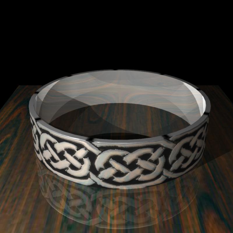
For the final part of the project, where I had to render a real object, I chose to render a Celtic ring that I wear. The image that you see below consists of a cylinder approximated by triangles with surface normals to provide smoothness. The complicated geometry for the Celtic knots is not modeled by triangles. Instead, a bump map has been applied to the flat cylinder. A total of 9 texture maps are used in the image, a diffuse map for the wood, and diffuse, specular, bump, and roughness maps for the outside and top of the cylinder.
Click the image for a larger version.
|