1	CS 248 Assignment 2 Polygon Scan Conversion CS248 Presented by Michael Green Stanford University October 20, 2004
2	Announcements… First thing: read README.animgui. It should tell you everything you need to know about the GUI. PLEASE post all questions to the newsgroup
3	Getting Started Read the project handout carefully! http://graphics.stanford.edu/courses/cs248-04/proj2.html Get the assignment from /usr/class/cs248/assignments/assignment2/ “README.files” goes over details on building the project, what different source files do, and where to find examples. “README.animgui” explains what to do once the program is running. How to create polygons, load/save object files, and create animations (we’ll go over most of this today too).
4	Development The interface is built using a cross platform library called GLUI. You won’t need to change the interface unless you add features (extra credit). In that case, see the GLUI manual in /usr/class/cs248/assignments/assignment2/arc. You can develop and test this program on Windows or Mac, just make sure it works on the Linux machines in Sweet Hall! When we give you the sample images, don’t worry about matching them exactly. Use the images to get an idea of correct behavior.
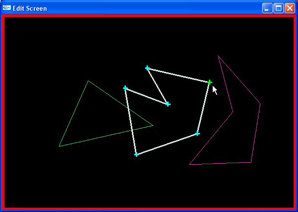
5	The Interface A few key points: (Shift + Left click) : add vertices. (Left click) : completes the polygon you’re editing, or allows you to select and drag vertices. (Right click) : drag the whole polygon The program we give you already handles all the editing functionality, you just need to work on the rendering.
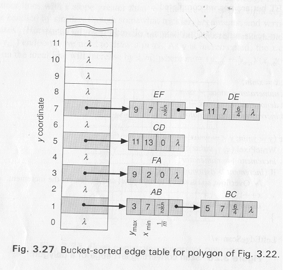
6	Scan Conversion (Rasterization) The Algorithm (page 98 in Computer Graphics FvDFH second ed.) Create an Edge Table for the polygon being rendered, sorted on y. Don’t include horizontal edges, they are handled by the edges they connect to (see page 95 in text).
7	Scan Conversion (cont.) Once you have your Edge Table (ET) for the polygon, you’re ready to step through y coordinates and render scan lines: 1. Set y to the first non-empty bucket in the ET. This is bucket 1 in the example. 2. Initialize the Active Edge Table (AET) to be empty. The AET keeps track of which edges cross the current y scan line. 3. Repeat the following until the AET and ET are empty: 3.1 Add to the AET the ET entries for the current y. (edges AB, BC in example) 3.2 Remove from the AET entries where y = ymax. (none at first in example) Then sort the AET on x. (order: {AB, BC}) 3.3 Fill in pixel values on the y scan line using the x coordinates from the AET. Be wary of parity– use the even/odd test to determine whether to fill (see next slide). 3.4 Increment y by 1 (to the next scan line). 3.5 For every non-vertical edge in the AET update x for the new y (calculate the next intersection of the edge with the scan line). Note: the algorithm in the book (presented here and in course lecture notes) attempts to fix the problems that occur when polygons share an edge, by not rasterizing the top-most row of pixels along an edge.
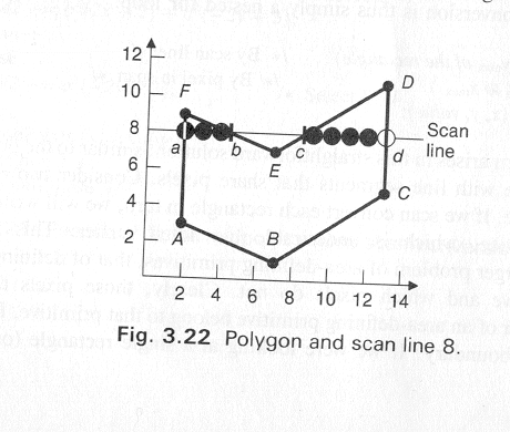
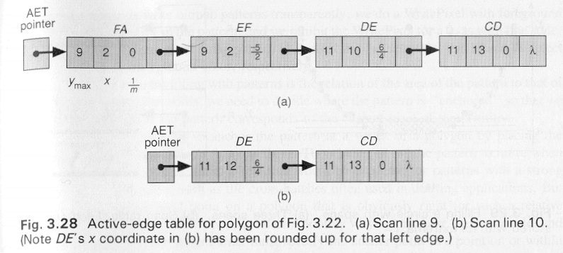
8	Active Edge Table Example Example of an AET containing edges {FA, EF, DE, CD} on scan line 8: 3.1: (y = 8) Get edges from ET bucket y (none in this case, y = 8 has no entry) 3.2: Remove from the AET any entries where ymax = y (none here) 3.3: Draw scan line. To handle multiple edges, group in pairs: {FA,EF}, {DE,CD} 3.4: y = y+1 (y = 8+1 = 9) 3.5: Update x for non-vertical edges, as in simple line drawing.
9	Active Edge Table Example (cont.) 3.1: (y = 9) Get edges from ET bucket y (none in this case, y = 9 has no entry in ET) “Scan line 9” shown in fig 3.28 below 3.2: Remove from the AET any entries with ymax = y (remove FA, EF) 3.3: Draw scan line between {DE, CD} 3.4: y = y+1 = 10 3.5: Update x in {DE, CD} 3.1: (y = 10) (Scan line 10 shown in fig 3.28 below) And so on…
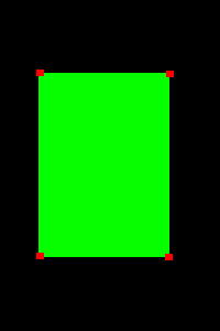
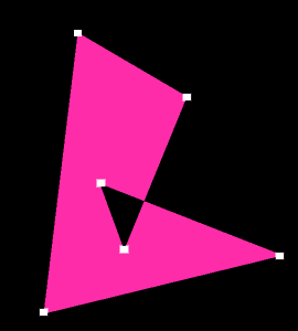
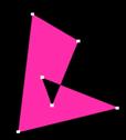
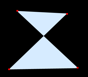
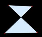
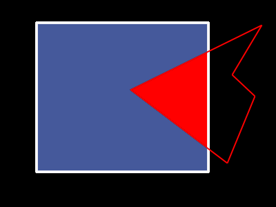
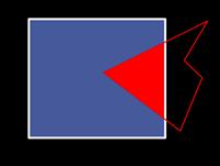
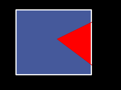
10	Test Images Some cases you should test:
11	Antialiasing Scan conversion with super-sampling. How can we achieve this? Two possibilities: 1. Scan convert once to a super-sampled grid, then average down. Cost: 1 scan conversion s² x p² storage, where there are (s x s) samples per pixel, (p x p) image s² x p² pixel writes 2. Perform many normal scan conversions at super-sampled locations, and additively combine them. You will implement this method using an accumulation buffer (coming up). Cost: s² scan conversions 2p² storage s² x p² pixel writes
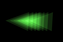
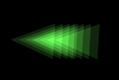
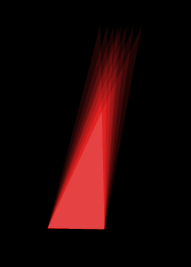
12	Motion Blur Synthesize the illusion that objects in our scene are moving quickly by blurring the image along the path of motion.
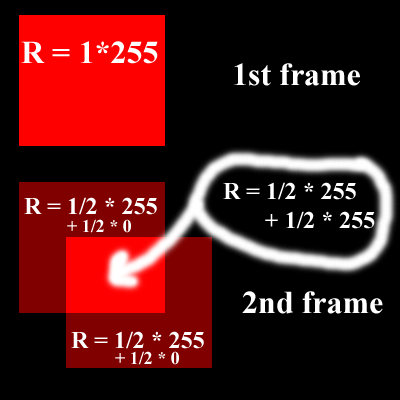
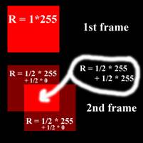
13	Accumulation Buffer Algorithm Allows us to successively render multiple “scenes” and have them additively blend as we go. Each image ends up with an equal weighting of 1/n, where n is the number of samples taken. (Appendix A in project 2 handout) Let "canvas" and "temp" be 24-bit pixel arrays. Let "polygon color" be a 24-bit color unique to each polygon. 1 clear canvas to black; 2 n = 0 (number of samples taken so far) 3 for (i=1; i<=s; i++) (for s subpixel positions) 4 for (j=1; j<=t; j++) (for t fractional frame times) 5 clear temp to black 6 n = n + 1 7 for each polygon 8 translate vertices for this subpixel position and fractional frame time 9 for each pixel in polygon (using your scan converter) 10 temp color <-- polygon color 11 for each pixel in canvas 12 canvas color <-- canvas color + temp color 13 canvas color <-- canvas color / n 14 convert canvas to 8x3 bits and display on screen (by exiting from your rasterizer)
14	Accumulation Buffer (cont.) Example (with overlap):
15	Accumulation Buffer (cont.) Question: Why should we render all polygons at once per frame (lines 7-10), why not antialias the objects separately and then blend their images together? Answer: Polygons on a perfect mesh over a colored background will show some of the background color. Rendering the polygons together prevents any unwanted blending.
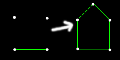
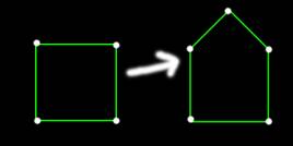
16	Extra Credit (Extra Credit is fun!!!) 1. Extend the interface to allow interactive scaling and rotations of polygons around a chosen point. Using matrices is one way… 2. Extend the interface to allow insertion and deletion of vertices in an already-defined polygon. Not hard mathematically, but think of usability as well. 3. Allow the number of vertices in a polygon to be different at any keyframe. Example: square to house.
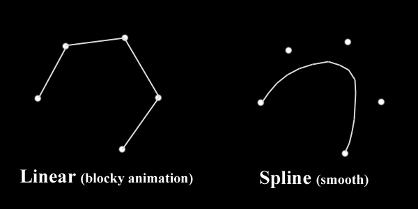
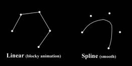
17	Extra Credit (cont.) 4. Extend the interface to allow the input of polygons with “curved” boundaries. Curve is approximated by lots of closely spaced vertices that are still linearly connected. Not too tough, add vertices along mouse path while mouse button is down. 5. Combine #3 and #4 to allow different curved boundaries for each keyframe. Calculate approximate locations for vertices when the number changes. For example, going from a curve with 10 vertices to one with 4, calculate points along the 4-vertex curve at 1/10 intervals. Or come up with a better scheme.
18	Extra Credit (cont.) 7. Define a “skeleton” of connected line segments, and replace (x,y) coordinates of vertices with (u,v) offsets from skeleton. Interpolate the skeleton, then use the offsets to calculate vertex positions. (draw sketch) 8. Implement polygon clipping. Scissoring means not sending pixel values to the canvas when they would be out of bounds (this is the required functionality). Full clipping means trimming the edge of the polygon so it fits within the screen, which can greatly reduce the time spent performing rasterization.
19	Extra Credit (cont.) 9. Implement unweighted area sampling (section 3.17.2 and earlier slide) as a user selectable alternative to accumulation buffer antialiasing (you must still implement accumulation buffer). For even more fun, implement weighted area sampling (section 3.17.3). 10. Create a cool animation and show it at the demo!
20	Development Tips Your canvas has (0,0) at the top left, with (canvasWidth-1, canvasHeight-1) at bottom right. Examples in book have (0,0) at bottom left. Doesn’t change too much, just be aware. If you are comfortable using them, you might find the C++ standard templates useful (especially sorted lists) for handling lists in your edge table. Alternatively, you might want to write your own class or functions to handle this.
21	Questions?