CS348B - Image Synthesis
Alan Jao
John Chin
Date submitted: June 8, 2005
|
|
|
Project Goal
The goal of the project is to accurately simulate the shape, color, and formation of the aurora borealis, or more commonly known as the "northern lights".
Motivation
The motivations for rendering this natural phenomenon are to provide aesthetic images for educational and entertainment purposes and to provide scientific value.
The aurora borealis is a natural phenomenon of great visual beauty and considerable scientific interest. It is one of the most fascinating and mysterious of nature's displays. The impressive visual characteristics of auroral displays have fascinated writers, philosophers, poets, and scientists over the centuries.
For any simulation of an environment typical of polar latitudes, the aurora is an obvious visual effect, and in fact it is often bright enough to navigate by or even to cast shadows. The aurora is also a strong visible effect in space, and even occurs on other planets with strong magnetic fields such as Jupiter.
In any effort in the physical sciences, models can be tested by how well their simulations predict observed data. Since the aurorae have such an obvious visual manifestation, reproducing their actual visual appearance is one way to evaluate auroral theories and data. The science behind the aurora is furthermore quite crucial because of its links to plasma physics.
Theory
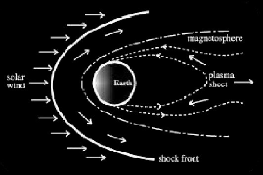
The Sun has an atmosphere and a magnetic field that extend into space. The Sun's atmosphere is made of hydrogen, which is itself made of subatomic particles: protons and electrons. These particles are constantly boiling off the Sun and streaming outward at very high speeds. Together, the Sun's magnetic field and particles are called the "solar wind."
This wind is always pushing on the Earth's magnetic field, changing its shape. This compressed field around the earth is called the magnetosphere. The Earth's field is compressed on the day side, where the solar wind flows over it. It is also stretched into a long tail, called the magnetotail, and points away from the Sun. Energy from the solar wind is constantly building up in the magnetosphere, and this energy is what powers auroras.
|
Solar particles are always entering the tail of the magnetosphere from the solar wind and moving toward the Sun. Now and then, when conditions are right, the build-up of pressure from the solar wind creates an electric voltage between the magnetotail and the poles.
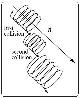
The voltage pushes electrons toward the magnetic poles, accelerating them to high speeds. Electrons in a magnetic field move in a special way: they are guided by the field. The electrons travel along magnetic field lines as if they were wires, circling around the lines in a long spiral as they go. They zoom along the field lines towards the ground to the north and south, until huge numbers of electrons are pushed down into the upper layer of the atmosphere, called the ionosphere.
In the ionosphere, the speeding electrons collide violently with gas atoms. This gives the gas atoms energy, which causes them to release both light and more electrons. In this way, the gases of the ionosphere glow and conduct flowing electric currents into and out of the polar region.
|
These electrons strike the gas molecules, which excites them to emit light. The color of the light you see depends on the type of gas. Every gas shines with its own special colors of light. These colors are like a fingerprint because no two gases give off exactly the same colors.
The unique colors of light produced by a gas are called its "spectrum". The auroral lights' colors are determined by the spectra of gases in the Earth's atmosphere, and the height at which the most collisions take place. Incoming particles tend to collide with different gases at different heights.
Very high in the ionosphere (above 300 km or 180 miles), oxygen is the most common atom, and collisions there can create a rare red aurora. The strong yellow-to-green light that is most common is produced by collisions with oxygen at lower altitudes, between 100 and 300 km. Around 100 km, nitrogen molecules produce a red light that often seems to form the lower fringes on aural curtains.
Lighter gases high in the ionosphere, like hydrogen and helium, make colors like blue and purple, but our eyes cannot always see them in the night sky. Good photographic film can be more sensitive to some colors than our eyes. Eyes see best in the green-yellow-orange part of the spectrum, where the Sun emits most of its light.
|
The basic shape of an aurora is determined by the energy and density of the electrons entering the atmosphere, as well as the local variations in the electric field of the Earth. The most basic aurora can be thought of as a "curtain" of light emissions from "sheets" of falling electrons.
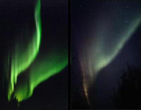
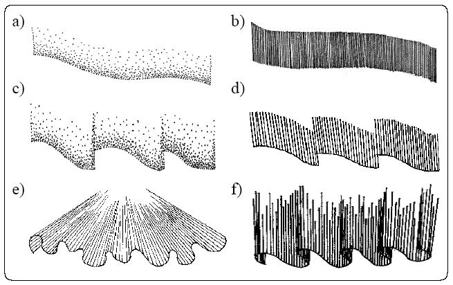
The auroral displays present a variety of forms when observed from the ground. In general, the auroral forms can be divided into two groups: those with and those without a rayed structure.
Among the auroral forms without a ray structure, we may find:
Among the auroral forms with a ray structure, we may find:
|
Technical Challenges
The key technical challenges of this project are roughly divided into two components. The first deals with the auroral shape and formation. The second deals with the auroral spectrum and intensity. Specifically, the tasks are:
Implementation
Our model of auroral shapes is based on the particle nature of the aurorae. However, instead of following the trajectories of individual electrons, we simulate the paths taken by beams of electrons. These beams represent auroral rays, or curls. This modeling approach is divided into two parts: the determination of the starting points for the beams and the simulation of their paths along the geomagnetic field lines.
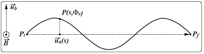
We modeled the shape of the aurora borealis as sheets with boundaries given by sine waves with a certain phase shift. Each sheet can be formed by several internal layers, and its shape defined by two parameters, the thickness, w, and the wavelength, lambda.
The boundaries as well as the internal layers of these sheets are modeled using sine curves. Hence, the starting points for the electron beams used in our simulations are obtained through the discretization of these curves. In our simulation strategy, folds are modeled by replacing portions of the sine waves by Bezier curves.
To calculate the electron beam starting point, we first need to determine the location of the starting point when projected onto a straight line path from the initial point to the final point of the sine curve. This is done by calculating the length of each starting point interval based on the number of starting points and wavelength and then modifying this value using a phase function to account for the different sine wave layers. This interval length is then modified using a random variable to model the stochastic nature of the aurora borealis.
After we have found the projected straight line location on the curve, we need to determine whether we are one the sine curve or the Bezier curve. To do so, we simply compare the location found above with the locations of the Bezier curves.
If the projected straight line location is on the sine curve, we can calculate its actual location on the sine curve using the sine function multiplied by an input amplitude parameter along the normal to the straight line connecting the initial and final points. The actual point is then the sum of two vectors, vector uA from the initial point to the projected straight line location and vector uB from the projected straight line location along the normal to the sine function value (see figure below).
If the projected straight line location is on a Bezier curve, we need to find the five Bezier control points since we are modeling folds with two loops. These five points are the start point(A), end point(E), midpoint of the start and end points(C), midpoint of the start and C point(B), and the midpoint of the end and C point(D).
With these five points, we then need to calculate the actual location on the Bezier curve. First, we calculate the intersection point between line AE and the normal to the straight line connecting the initial and final points of the sine curve. Second, we determine which fold of the Bezier curve the intersection point lies on. Third, we calculate the parametric t value of the intersection point. Finally, we plug t into the Bezier curve equation P0(1-t)^2 + P1(2)(t)(1-t) + P2(t)^2.
The electrons are randomly deflected after colliding with the atoms of the atmosphere. These deflections play an important role in the dynamic and stochastic nature of the auroral display and are thus taken into account in our simulations. We consider the deflection points as emission points and they are used to determine the spectral and intensity variations of the modeled auroral displays.
To simulate the path of electrons along the geomagnetic field lines, we first need to determine the location of the collision point when projected onto the magnetic field line path. This is done by calculating the length of each collision interval based on the number of collisions and the height. This length is then modified using a random variable to model the stochastic nature of the aurora borealis.
After we have found the projected straight line location on the curve, we generate a random azimuthal angle to perturb the z coordinate of the electron beam. The actual collision point is then the sum of two vectors, the vector from the last collision point to the projected straight line location and vector uB from the projected straight line location along the normal to the Bezier function value.
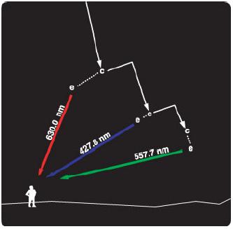
As explained previously, the color spectrum emitted from the aurora borealis are dependent on the type and the energy of the particles that collide with the precipitating electrons. These two factors are statistically dependent on the altitude. Empirical evidence shows that spectral appearance of the borealis are mainly due to the emission of light in the following three wavelengths: 630.0nm, 557.7nm, and 427.8nm. Color in these three wavelength are roughly red, green, and blue, respectively.
The spectral variety of the auroral displays is further contributed to by several weaker light emissions at other wavelengths across the visible spectrum. However, these weaker emissions are not obvious for the casual observers. Therefore, in the implementation, we focuses only on emission profile of the three major frequencies stated. The figure below shoes the spectral distribution for the three wavelengths between 100 to 300 kilometers above the ground.
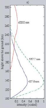
In the implementation, a lookup table is built using the functions shown in the above figure. The lookup table is constructed by taking samples from each of the three functions at discrete steps along the y-axis. The range from 100 to 300 kilometer are divided into 100 segments, resulting in a set of 101 samples for each function, which is sufficient for the purpose of the simulation.
After obtaining the lookup table. The height values in which these values are at are normalized from [100, 300] to [pMin.y, pMax.y] where pMin.y and pMax.y corresponds to the minimum and the maximum y values of the bounding box for the borealis in the object space. These bounding box vertices are computed by the aurora shape computation code described in the previous two sections.
The lookup table approximates the functions by using linear interpolation for the query point between the sample points. After obtaining the values for the three frequencies, we must convert it into the standard RGB values. This is done by first converting the values into CIE XYZ color space, using the coefficients provided by pbrt, and then convert them to standard RGB space from XYZ space.
The light intensity from an aurora is proportional to the deposition of energy into the atmosphere by the precipitation electrons. As a result, the height and the intensity distribution of each auroral form are related to the average energy distribution of the particles. The intensity distribution of several aurora form are shown in the plot below.
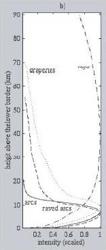
The x-axis shows the normalized intensity, whereas the y-axis shows the height relative the the bottom of the aurora sheet. Upon observation, these functions are similar in shape to a family of functions called the lognormal distribution function. The lognormal distribution function are probability density function of the form
|
|
where ![]() is
the shape parameter,
is
the shape parameter,
![]() is the location parameter and m is the scale parameter. The
case where
is the location parameter and m is the scale parameter. The
case where
![]() = 0 and m = 1 is called the standard lognormal distribution. In the
function fitting process, the standard lognormal distribution function is used,
with the shape parameter
= 0 and m = 1 is called the standard lognormal distribution. In the
function fitting process, the standard lognormal distribution function is used,
with the shape parameter
![]() =1 since the
resulting shape closely matches the one shown in the figure.
=1 since the
resulting shape closely matches the one shown in the figure.
In order to parameterize the standard lognormal distribution to fit all the intensity functions shown above, we define a new function
![]()
with parameters a and p, where a is used to scale the intensity values and p is used to modify the intensity falloff rate with height.
The technique used in the rendering of the borealis is similar in spirit to that of volumetric photon mapping. The rendering of the borealis in pbrt is done in two stages. In the first stage, the shape model of the borealis described is used to generate all the collision points of the precipitating electrons in object space. These positions are then passed into a 3D KD-tree to build an electron map for the borealis sheet, along with its bounding box vertices.
In the second stage, we treat the borealis in pbrt as a volume of participating media, with variable density and emission but zero scattering and absorption properties. After constructing the electron map, we approximate the variable densities of this volume by keeping track of a collection of density values at regular grid points inside the bounding box. These density values are computing by utilizing the proximity lookup capability offered by the KD-tree structure. After obtaining the densities at the grid points, trilinear interpolation can be used to compute the densities at any arbitrary points inside a 3D grid voxel.
The spectrum and intensity at a given point inside the volume is computed by using the lookup table and the lognormal distribution, respectively.
Now having able to compute the density, spectrum, and intensity at any query position, the resulting color emitted at that position due to the borealis at that position is simply the product of the density, intensity and spectrum. Now given an eye ray that goes through the volume, the total light emitted along the direction of the ray is simply calculated by approximating the total optical thickness of this volume with respect to that ray.
Results
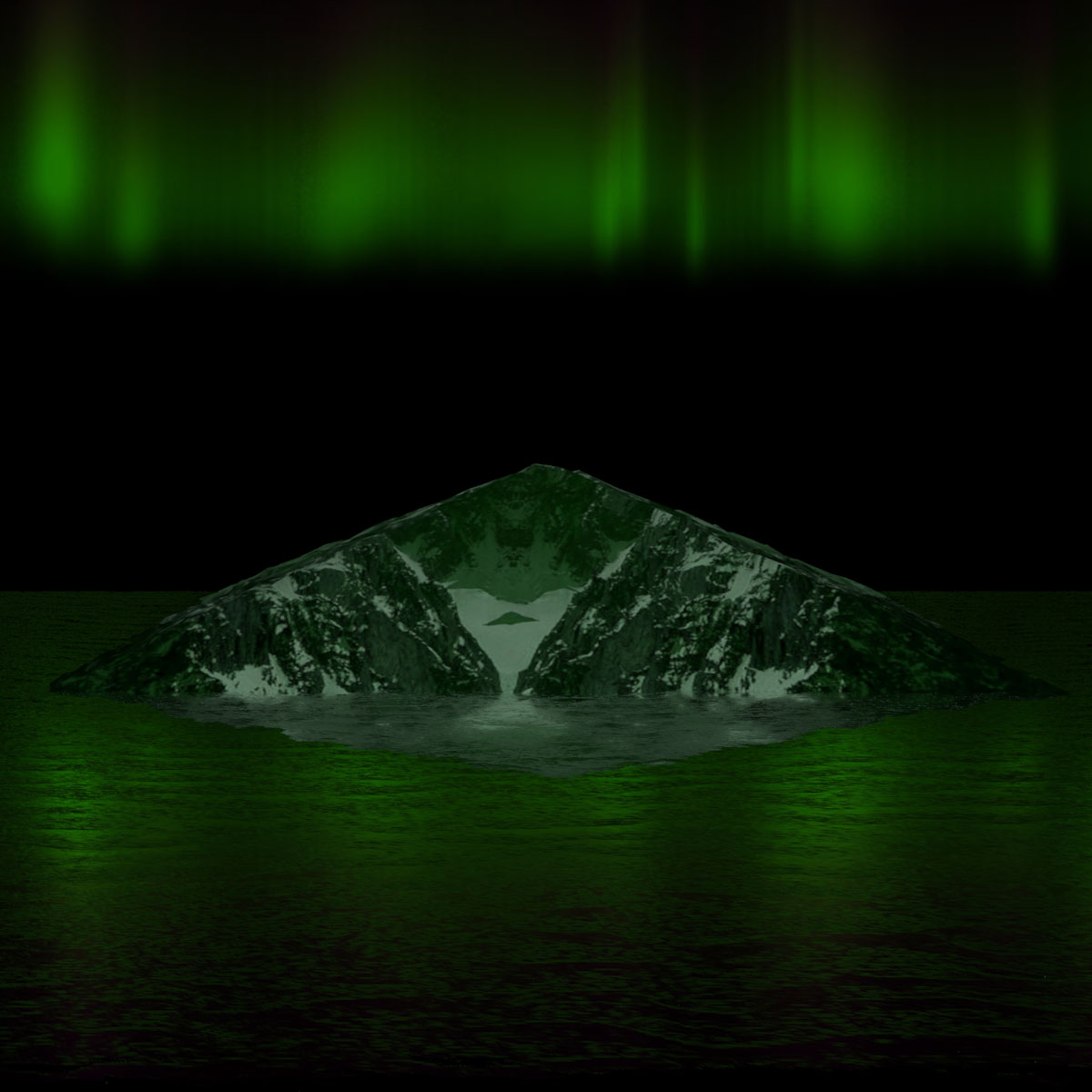
The results of our implementations are shown below:
|
Simulating the arc aurora form without ray structure (figure a from theory
section). This type is characterized by the narrow band height, with
no red band region:
|
|
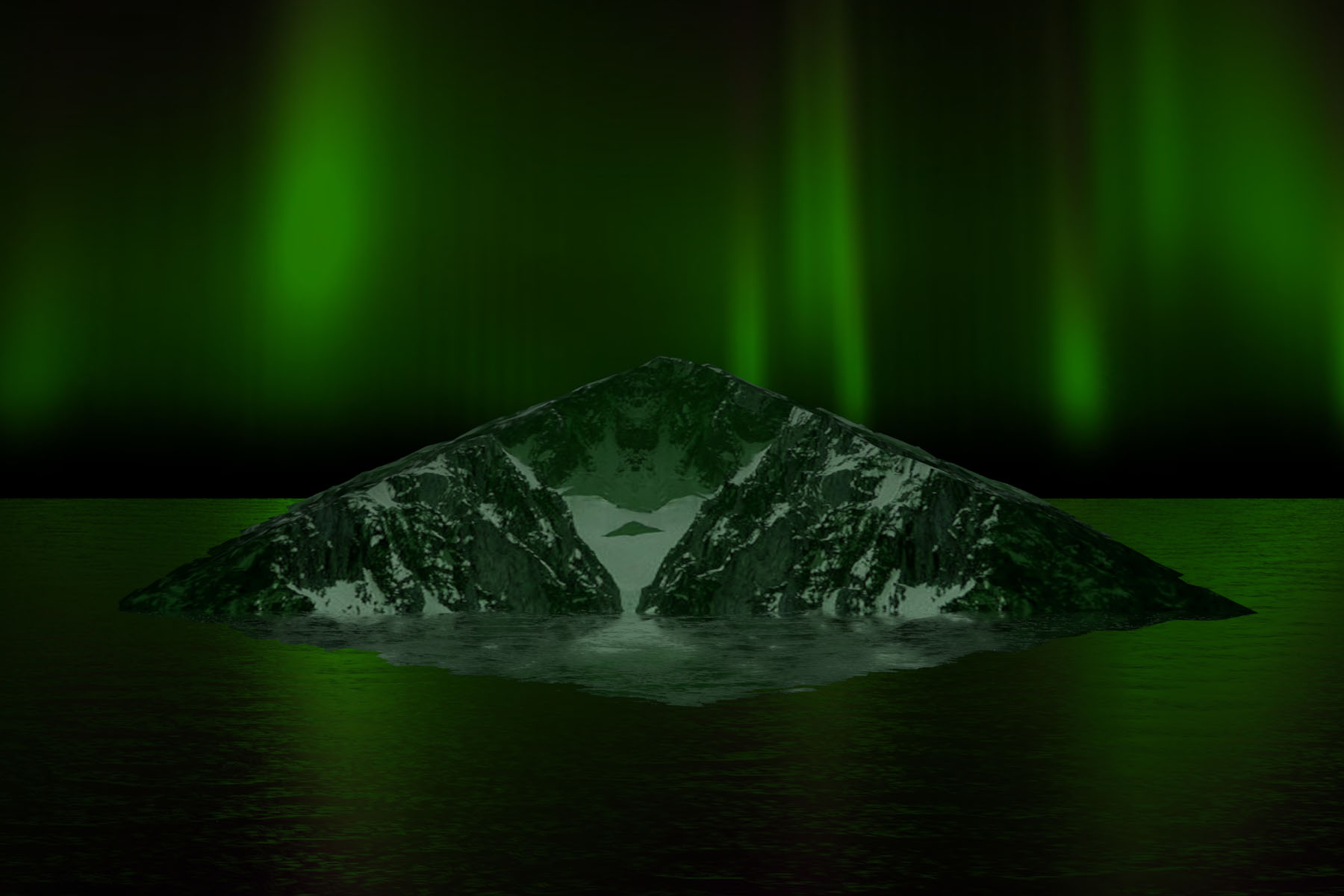
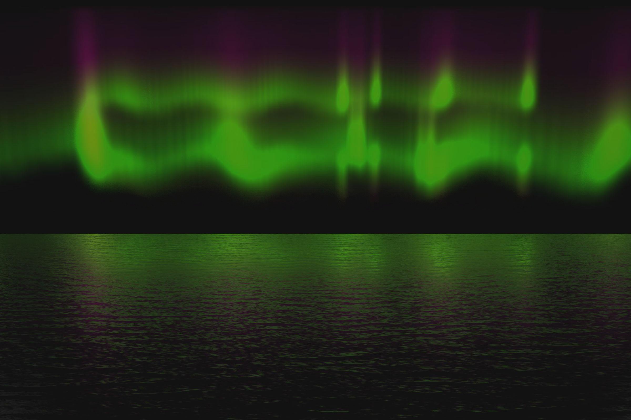
Simulating arc aurora form with ray structure (figure b from theory
section). This type is characterized by the wider band height, with
slight red band region on the top:
|
|
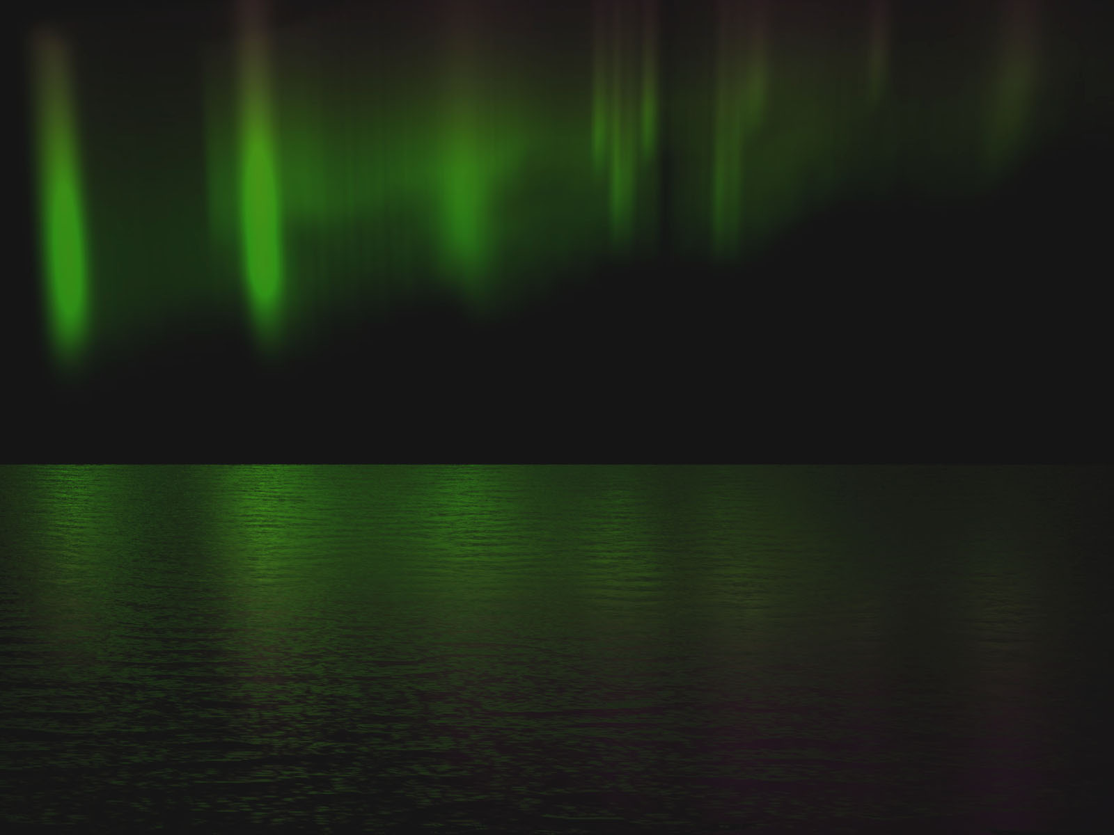
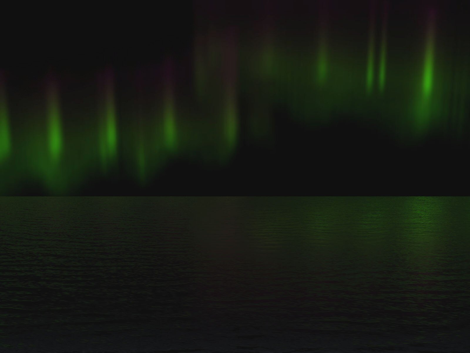
Two more arc aurora images (with folds):
|
|
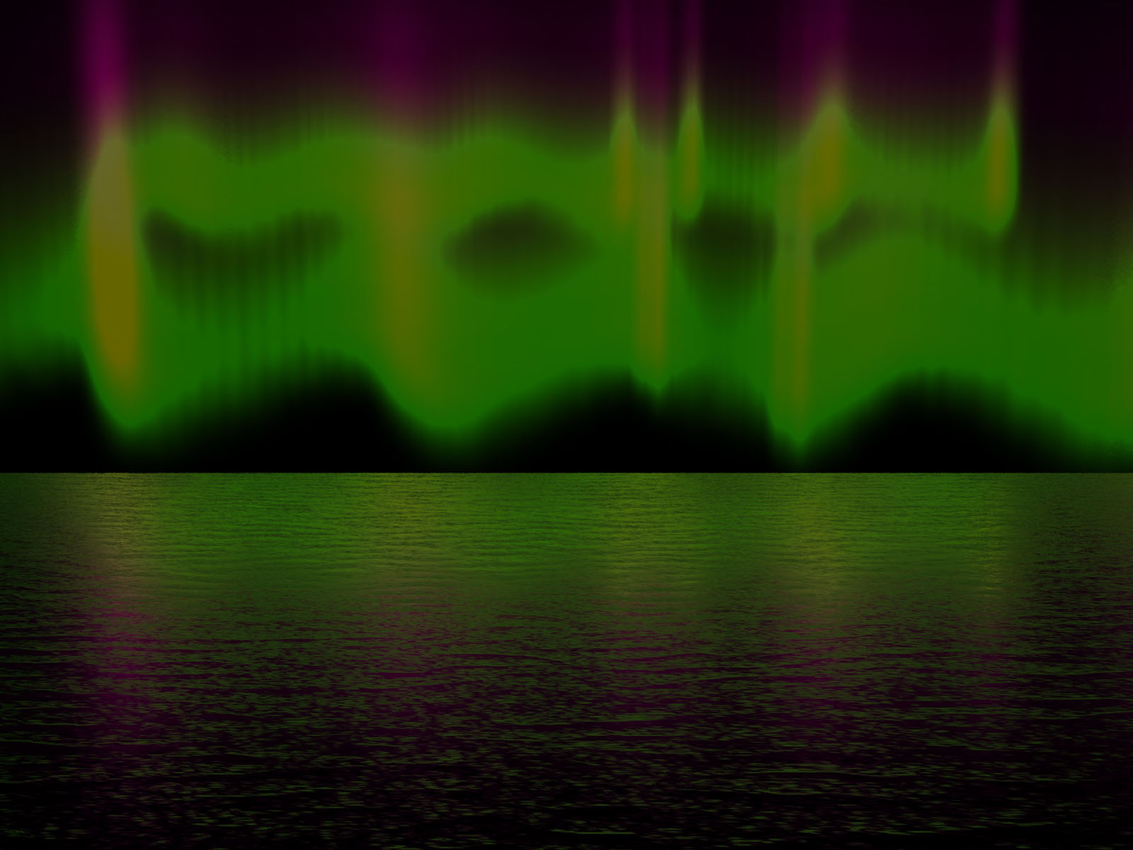
Simulating drapery aurora form (figure f from theory section) with folds.
This type is characterized by the wide band height and intense emission,
with thicker red band region on the top:
|
Conclusion
The models of borealis and the rendering techniques used in this project
provides satisfactory results in terms of simulating statically the basic
structure of borealis, namely the arcs and the folds, as well as its spectral
emission and intensities for various different types of the aurora form, as seen
from the results section. However, what is modeled is inadequate to
simulate the more complex behaviors of aurora such as curls and spirals, which
is closely related to the dynamic variation of the aurora borealis with respect
to time. In order to simulate the transformation of the borealis shape
through time requires modeling the dynamics of the aurora sheet, which is not
captured in the model presented in this project. This extension in
modeling is left for future work.
References
[1] BARANOSKI, G., RONKE, J., SHIRLEY, P., TRONDSEN, T., AND BASTOS, R.
Simulating the Aurora Borealis