Redwood Trees in Fog
CS348b Rendering Project Final Report, June 2005
Andrew AdamsEmilio Antunez
Eino-Ville Talvala
Introduction:
We
were interested
in generating a realistic rendering of a redwood forest in fog, with
special attention paid to the bark surface, undergrowth foliage, and
the patchy, clinging fog. See our original project proposal here.
Result:
The
final image is at 1600x900 pixels, with 10 samples per pixel.
The standard single scattering volume integrator and the direct
lighting surface integrator were used for the scene.
The total render time was 48 CPU-hours on 3 Athlon 64 3000+ machines with 1 GB of RAM.
The projector light source was used to add dappled light beams into the scene, and a trianglemesh generated with multifrequency noise and covered with a bark chip texture was used for the ground. All of the major elements of the scene are described below in detail.
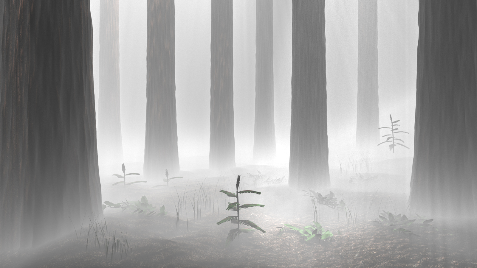
Click image for full 1600x900 image. EXR Version: forest_final.exr
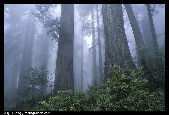
Inspirations:
These are the images we used as a starting point for the look we were after.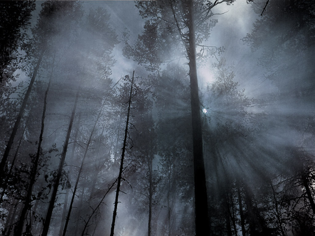
Interesting parts:
- Redwood tree trunk generation - Andrew
- Foliage and undergrowth generation - Emilio
- Clinging fog calculation - Eino-Ville
Redwood trunks:
AndrewCreating
the tree
trunk surfaces is an exercise in controlled noise. We need to create a
map for radius and for theta, which will give us a large cylindrical
mesh.
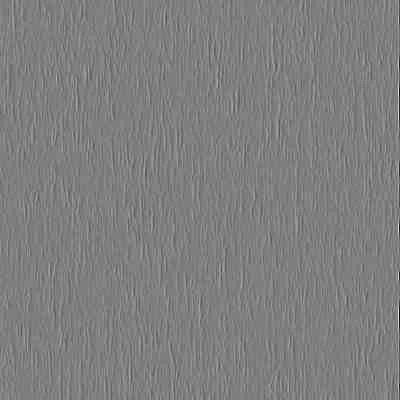
We start with a method for producing fissures. This operates on an initially uniform gray map of probabilities. A randomly selected point is either selected as fissure or not fissure, according to the probability value there. The probabilities for neighbours within a 5x7 window around the pixel are then altered. In either case, neighbours in the horizontal direction become less likely to make the same decision, and vertical neighbours become more likely to make the same decision.
Running this until most pixels have made a decision produces a fairly good map of fissuring, in a restricted range of frequencies. Here is such a map upsampled to 400x400.
Low-frequency fissure map
To
add fissures at
other frequencies, we repeat the algorithm on a pyramid of initially
gray images, taking a geometrically weighted sum of the results,
favoring lower frequencies.
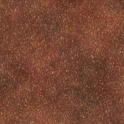
Adding higher frequencies to fissure map
This nearly gives us our final map of radius. All that remains is to flare out the base of the trunk. This is done by adding a random selection of sin curves with amplitude inversely proportional to frequency and height above the ground.
We start with a uniform gradient image for our map of theta. We wish to exaggerate the concavities already present in the radius map, so we add to this the horizontal derivative of the absolute value of the horizontal derivative of the radius map. This function has the following effect on points.
Below is the theta offset map for the above noise.
The actual amount we modify theta by is quite small, as shown by the final theta map, which is nearly a smooth gradient.

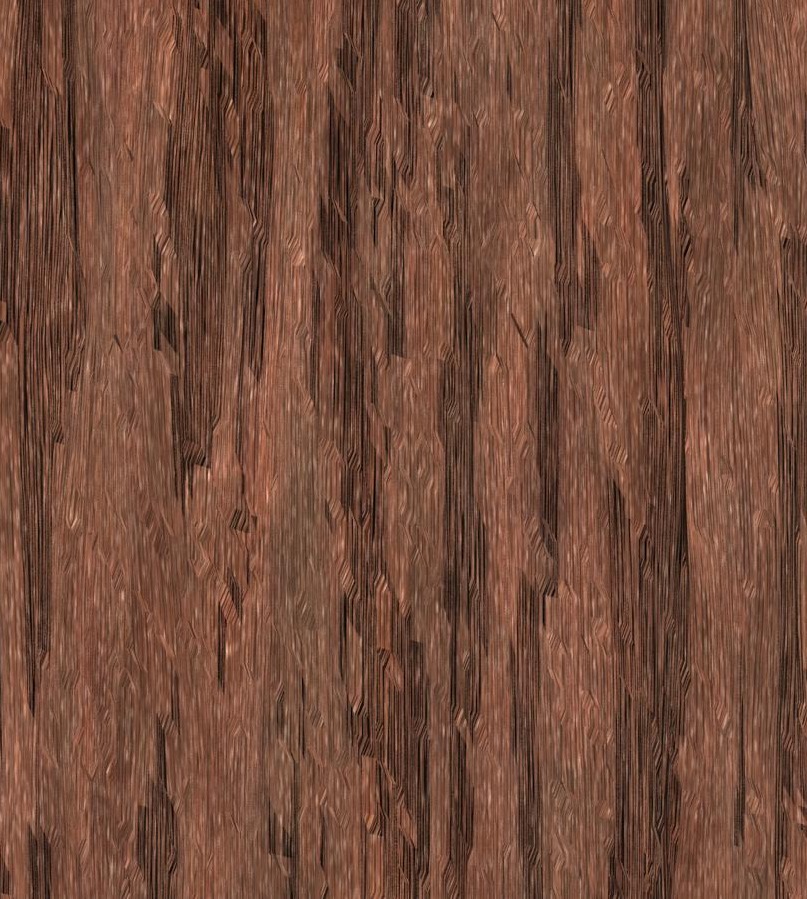
These maps determine the geometry of our tree trunk. To this we add a texture map. The texture is generated as geometrically weighted pyramid of noise in 3 channels, which is then used to linearly interpolate between red, brown, and gray. To this small vertical flecks are added to simulate lichen and hanging splinters of bark. The texture map is stretched vertically when it is applied to the tree geometry.
The tree is also given a bump map, which is random noise stretched vertically by a factor on the order of 100. These effects all add to produce the bark image shown below, which is taken from the top left corner of the final image without fog.
Adding higher frequencies to fissure map
This nearly gives us our final map of radius. All that remains is to flare out the base of the trunk. This is done by adding a random selection of sin curves with amplitude inversely proportional to frequency and height above the ground.
We start with a uniform gradient image for our map of theta. We wish to exaggerate the concavities already present in the radius map, so we add to this the horizontal derivative of the absolute value of the horizontal derivative of the radius map. This function has the following effect on points.
Below is the theta offset map for the above noise.
The actual amount we modify theta by is quite small, as shown by the final theta map, which is nearly a smooth gradient.
These maps determine the geometry of our tree trunk. To this we add a texture map. The texture is generated as geometrically weighted pyramid of noise in 3 channels, which is then used to linearly interpolate between red, brown, and gray. To this small vertical flecks are added to simulate lichen and hanging splinters of bark. The texture map is stretched vertically when it is applied to the tree geometry.
The tree is also given a bump map, which is random noise stretched vertically by a factor on the order of 100. These effects all add to produce the bark image shown below, which is taken from the top left corner of the final image without fog.
REFERENCES:
[Sylvain 2002]Sylvain Lefebvre and Fabrice Neyret, "Synthesising bark", Eurographics 2002
Foliage:
EmilioOne
of the major technical challenges of the project was to create
convincing plants for ground cover in the image. This was accomplished
by implementing a parametric 0L-system parser, similar to the
one described by [Prusinkiewicz 03], with the addition of randomized
parameters.
The parser takes in a context-free grammar that describes the rough structure of the plant. Each symbol of the grammar is allowed to have one associated floating-point parameter.
The parser starts with an "axiom" (an initial string) explicitly given by the user, and expands this word on every iteration using the productions of the grammar. Each symbol may have several productions, each of which have an associated parameter range. Assuming these ranges are disjoint, the l-system can determine which production to apply to a symbol based on that symbol's current parameter value.
In addition to specifying the new symbols to replace an old symbol, each production must also specify a parameter to go with each new symbol. (If a parameter is not explicitly given, it is assumed to be "0"). The parameter can be described as any linear combination of the old symbol's parameter ("s"), a random U[0,1] parameter ("r"), and a constant.
A sample production would be
A(s) {1,10} -> B(s*2) C(5) D(r) E(s*5.5+r*2-10)
This says that A gets expanded to the string BCDE (with the given parameters) when A's parameter "s" is between 1 and 10 (inclusive).
Once a grammar is defined, the l-system is run through an arbitrary number of iterations to generate a sample plant structure, and is saved to a file. This file is then fed to a plant modeling program, which creates an appropriate PBRT model from it.
In defining the l-system grammar, a few symbols are reserved for explicit commands to the modeler. In particular, six symbols (+,-,&,^,/,\) are reserved to define curvature commands for the plant's stem, two symbols (#,!) are reserved to specify increments/decrements to the stem width, f(s) is used to draw a stem segment of length s, and l(s) is used to draw a leaf at scale s. Note that these are the only symbols that are read in by the modeler (and they are the only ones needed).
The modeler creates a PBRT file by taking the l-system output, as well as an explicit model for a leaf and a stem segment. The leaf and stem segment models are defined as objects, and then instantiated repeatedly in the full plant model.
The resulting plants can be quite convincing, as seen in the test images. The randomized parameter in particular makes a big difference, since it allows organic-looking growth of the plant without requiring the definition of a massive, complex grammar.
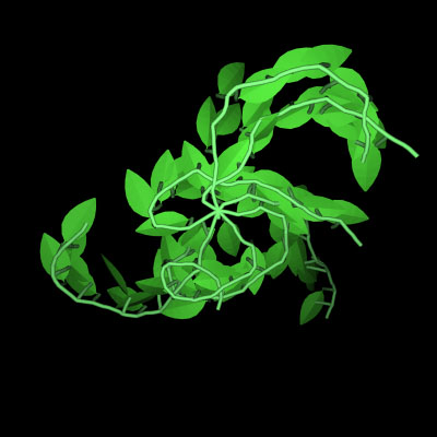
A view of a ground vine from below
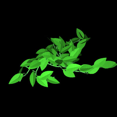
Same vine from the front
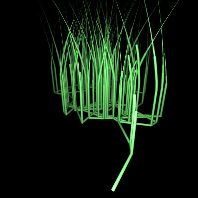
A grass model - Note that the 'roots' are below ground on the final renders
REFERENCES
[Prusinkiewicz 03]
Prusinkiewicz, P., Hanan, J., Hammel, M., Mech, R., "L-systems: from the
Theory to Visual Models of Plants," Course notes from SIGGRAPH 2003.
[Smith 84]
Smith, A.R., "Plants, Fractals, and Formal Languages," ACM SIGGRAPH
Computer Graphics, Proceedings of the 11th annual conference on computer
graphics and interactive techniques, Volume 18 Issue 3, January 1984.
Fog:
Eino-VilleThe
goal for the
fog was to create a variable-density fog region, where the fog was
thicker along the ground, as well as clinging to the trees.
In general, this requires the fog density to be a function of the
distance to both the ground (a trianglemesh or a heightfield) and the
surrounding tree surfaces.
Initially, I planned to implement the shell mapping technique from a paper to be published at Siggraph 2005, by Porumbescu et al: Shell Maps(PDF). A shell map is an extension of a standard two-dimensional texture, where an offset surface is generated for a triangle mesh object, and the volume enclosed by the original mesh and the offset surface is subdivided into tetrahedra. Combined with a UV map of the original surface, the tetrahedra can then be used to map a slab of UVW texture space to the space surrounding the object in a consistent piecewise-linear mapping. For the forest scene, I planned on generating the union mesh of the ground and the tree trunks in the scene, and then expanding the offset surface as much as possible without self-intersection, in order to cover all of space within the shell map and establishing a UVW mapping of all space that related to the scene geometry well.
As in the original paper, I used the offset surface generation code from UNC Chapel Hill [Cohen 96]. The offset surface maintains a 1:1 correspondence between original mesh surface vertices and offset surface vertices, which allows for the generation of triangular prisms from corresponding surface and offset surface triangles. Since the triangular prisms are not guaranteed to be convex, they cannot directly be used to map between shell space and texture space. Instead, they must be split into 3 tetrahedra each, while keeping the splits consistent - that is, two matching faces on two prisms must be split along the same line to guarantee a continuous mapping across the face. Below is the wireframe of the constructed tetrahedral mesh around the Stanford bunny, with a closeup:
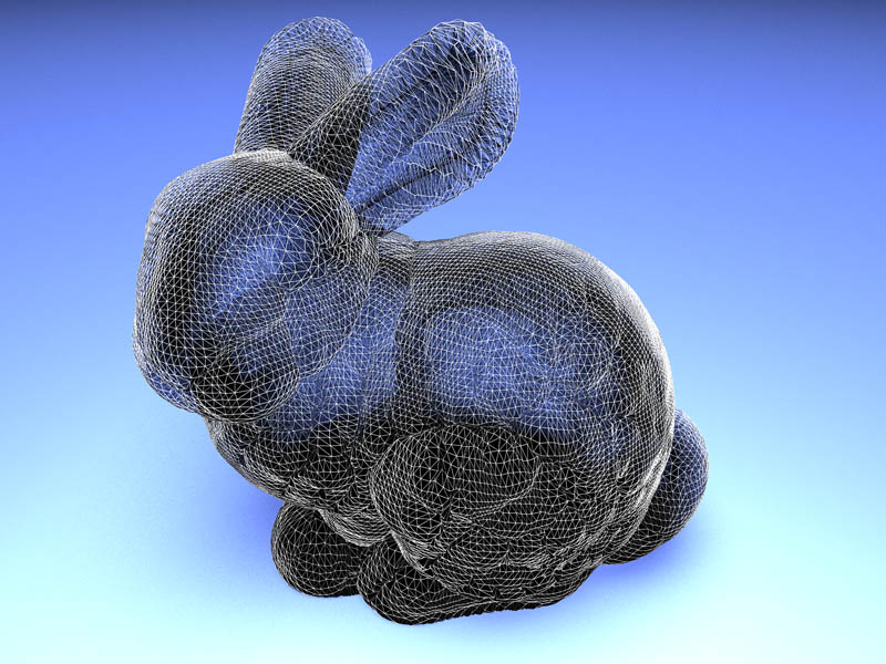
Tetrahedral shell map surrounding the Stanford bunny
Initially, I planned to implement the shell mapping technique from a paper to be published at Siggraph 2005, by Porumbescu et al: Shell Maps(PDF). A shell map is an extension of a standard two-dimensional texture, where an offset surface is generated for a triangle mesh object, and the volume enclosed by the original mesh and the offset surface is subdivided into tetrahedra. Combined with a UV map of the original surface, the tetrahedra can then be used to map a slab of UVW texture space to the space surrounding the object in a consistent piecewise-linear mapping. For the forest scene, I planned on generating the union mesh of the ground and the tree trunks in the scene, and then expanding the offset surface as much as possible without self-intersection, in order to cover all of space within the shell map and establishing a UVW mapping of all space that related to the scene geometry well.
As in the original paper, I used the offset surface generation code from UNC Chapel Hill [Cohen 96]. The offset surface maintains a 1:1 correspondence between original mesh surface vertices and offset surface vertices, which allows for the generation of triangular prisms from corresponding surface and offset surface triangles. Since the triangular prisms are not guaranteed to be convex, they cannot directly be used to map between shell space and texture space. Instead, they must be split into 3 tetrahedra each, while keeping the splits consistent - that is, two matching faces on two prisms must be split along the same line to guarantee a continuous mapping across the face. Below is the wireframe of the constructed tetrahedral mesh around the Stanford bunny, with a closeup:
Tetrahedral shell map surrounding the Stanford bunny

Closeup of ear of bunny shell map
However,
even
though the construction of the shell map is not time-intensive, using
it for volume rendering is far more so. To render a
volumetric ray with a single scattering bounce (The singlescattering
volume integrator in PBRT does this), we now need to step along the ray
in the texture space, where the ray is piecewise linear. This
means that in the world space, we must find all the tetrahedra that are
intersected by the ray, transform each intersection segment into UVW
space, obtain the transmission and illumination of the volume within
each UVW ray segment, and then finally combine all the segment's
transmission and luminance values together. The primary cost
here is to find the original ray-tetrahedron intersections. I
used the PBRT built-in octree data structure, adding the ability for
the structure to handle ray intersections, to intesect the ray with the
shell map tetrahedra. However, this was still a slow process,
with the intersection tests taking several times the time of the actual
transmission calculations, and comparable time to the incoming
luminance calculations. Attempts to traverse the
shell map data structure itself for tracking the ray ran into
difficulties with numerical accuracy when a ray barely entered a
tetrahedra (where the entering and exiting times were within the
floating-point accuracy of the system and thus not sortable) or when
the ray's maxt point corresponded to the inner surface of the shell map
and the determination of whether the ray ended inside the tetrahedron
was not numerically stable. The second case was especially
common, since the inner surface of the shell map is equivalent to
geometry in the scene, and thus commonly represents the endpoint of a
ray. As a result of all of the above, we determined that the
shell map would simply be far too slow to work for a more complex
scene. Below is the only succesful image of shell-mapped fog
we generated. The underlying fog is simply an exponential
falloff fog, a default PBRT plugin. It is wrapped around a
simple C-shaped triangle mesh:

Shell-mapped fog around a C-shaped mesh
My
second approach
is far more scene-dependent, but worked far faster. I
implemented a new volume region, forestfog, inheriting from the default
PBRT densityregion class, which contains basic code for handling a
variable-density fog field. Given all of the scaffolding
provided by PBRT, all I needed to implement was a function describing
the fog's density at a given point P in the world. As a first
attempt, I simply passed the world coordinates of each tree trunk's
center into forestfog. Inside the density function, I
deteremined which tree trunk was closest to P, and used the distance to
the tree's center as a height variable for an exponential fog
distribution. Below is an image of the result in a test scene:
Cylindrical-density fog
While
this method
does clump fog around the tree trunks, the fog does not truly follow
the tree surface. In order to have the fog be a function of
true distance to the tree, I decided to cast a ray from P toward the
closest tree center, and use the distance to the first intersection as
the distance to the tree surface. Since ray casts are
expensive, I only cast the ray if I am within a threshold distance of
the tree center - otherwise I simply use the center distance, minus an
average tree radius, as the distance to the tree surface. I
also included a transition region in which I linearly blend from the
cylindrical approximation to the true raytraced distance
function. This approach works well, since far away from the
tree small surface variations have little impact on fog
density. Below is an image generated using ray-cast surface
distance fog. As is clear, the fog now clings along the tree
surface well.

Ray-cast surface distance fog
Finally,
I added
height above ground to the density function. Since the
heightfield has significant variation in the scene, I did not use a
height approximation far away from the ground. Instead, a ray
is always cast downward from P in order to determine the closest
surface below P. Note that this has an additional benefit in
that the ground foliage is also used in the density determination - the
fog will appear to cling to the topsides of foliage as well.
Combining all this into a single density function, I obtained the
equation:
Density(P) =
a*exp(-b*Distance_to_tree_surface(P)-c*Height(P)) + d*exp(-e*Height(P))
+ f
The
constants a
and d control the fog thickness right at the ground and tree
surface. The constants b, c, and e control the rate
of fog dissipation with height and distance from the tree surface. The
final constant f is used to set up a base level of homogenous fog
throughout the scene. Note that the tree surface fog is also
modulated by height, so that fog does not cling with equal density all
the way up the tree, but instead disappears at some point.
Below is a test image generated with this fog function:

Final fog density function test image
REFERENCES
[Porumbescu 05]
Serban D. Porumbescu, Brian C. Budge, Louis Feng, Kenneth I. Joy, "Shell Maps," To be published in Proceedings of ACM Siggraph 2005.
[Cohen 96]
Cohen, Jonathan, Amitabh Varshney, Dinesh Manocha, Greg Turk, Hans Weber, Pankaj Agarwal, Frederick Brooks, and William Wright. "Simplification Envelopes," Proceedings of SIGGRAPH 96 (New Orleans, LA, August 4-9, 1996).
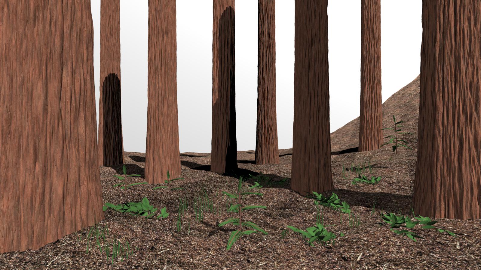
Below is a version of the image with no fog and simple lighting, useful for seeing the detail in the geometry. Click for full size