Final Project
Group Members
Christina Chan
Crystal Fong
Project Proposal
Our final project proposal can be found at CrystalFong/FinalProjectProposal
Overview
The goal of our project is to render an underwater scene of clownfish and sea anemone. To achieve this, we implemented two different subsurface scattering techniques to simulate the glowing and lighting of an underwater image.
Reference image
|

Approach
Fish (Christina)
Model
The fish model used in the project was acquired from the web (http://toucan.web.infoseek.co.jp/3DCG/3ds/FishModelsE.html). We used the wavefront pbrt plug-in provided by Mark Colbert to load the model. Since different segments of a fish display different material properties, we had to separate the model into parts. This is done by parsing the OBJ file, and noting the discontinuities in the model.

In order to simulate the texture of a fish, we attempted to create a scale model and procedurally cover the fish body with it. However, that gave a clumpy appearance, and significantly increased the rendering time. We therefore decided to apply bump mapping to the body and the fins instead.
Scale model:

Sphere covered with scales:

Fish body covered with scales:

Bump map texture for fish body:

Techniques
To accurately simulate the transparency and the reflective behavior of fish scales, and the softness of fish fins, we implemented the thin film subsurface scattering method described in the “Reflection from Layered Surfaces due to Subsurface Scattering” paper. Because of the thinness of scales and fins, we used a first order approximation, which assumed single scattering event. To implement this, we created two BxDF subclasses, one for reflection and one for transmission.
In the reflection model, the radiance included two terms, one for surface reflection and one for subsurface reflection, and the terms are weighted according to the Fresnel coefficients:
- f_r= R*f_r,s + (1-R)*f_r,v
Backscattered radiance is computed using the following equation:
- L_r,v(theta_r, phi_r)= W*T12*T21*phase*cos(theta_i)/(cos(theta_i)+ cos(theta_r))*(1-exp(-tau_d*(1/cos(theta_i)+ 1/cos(theta_r)))*L_i(theta_i, phi_i)
where the phase function is estimated using the Henyey-Greenstien formula:
Phase= (1/4*pi)*(1-g2)/(1+g2-2*g*cosj)^(3/2)
The parameters used are close to those of epidermis given in the paper. The mean cosine of phase function (g) was varied according to the part of the fish. For example, scales are more reflective than fins and thus have a smaller g to give higher backscattering.
In the transmission model, the forward scattered radiance is given by
- L_t,v(theta_t, phi_t)= W*T12*T23*phase*(cos(theta_i)/(cos(theta_i)-cos(theta_t))*(exp(-tau_d/cos(theta_i)- exp(-tau_d/cos(theta_t))*L_i(theta_i, phi_i)
In the case where cos(theta_t)==(cos(theta_i)), the following equation is used to avoid singularity:
- L_t,v(theta_t, phi_t)= W*T12*T23*phase*tau_d/cos(theta_t)*exp(-tau_d/cos(theta_t))*L_i(theta_i, phi_i)
The following is a test image of the fish rendered using thin film subsurface scattering:

As shown in the figure, the fish body is too tranparent if rendered using only first order thin film subsurface scattering because of the high translucency of the fish scale material. To solve this, we added an additional layer inside the fish body that is rendered using the Translucent material class. This layer represents the flesh of the fish and gives a much more solid look to the fish.
Technical Challenges
One of the challenges of creating a realistic rendering of a clown fish is to get the textures right. All texture maps (including color textures and bump map textures) were created in Photoshop. Surprisingly, it was very difficult to get the textures right due the stretching effect during texture mapping. In hindsight, we should have modified the wavefront pbrt plug-in to obtain texture coordinates. The following is the color map used for the fish body:

Anemone (Crystal)
Model
The anemone model was procedurally generated using a python script to create a scene file. Each anemone stalk has a Catmull-Rom spline as a backbone, and is modeled using generalized cylinders (see the Resources section for a link to a tutorial). The script takes a control point list as input to set the initial spline curvature. To interpolate one point, it is necessary to have 4 control points (2 on each side of the desired point.) Intermediate points are generated using the following equation where p_i is a control point and t is a value between 0 and 1 that represents the distance of the desired point from the second (P1) point (where t=0 is at P1 and t=1 is at P2).
q(t) = 0.5 * ((2 * P1) + (-P0 + P2) * t +(2*P0 - 5*P1 + 4*P2 - P3) * t2 + (-P0 + 3*P1- 3*P2 + P3) * t3)
At each point(q), we calculate and store the normal(N), tangent(T) and binormal(B). This is accomplished by the following steps.
- For the very first point, select T, N, and B.
- For each point Q1:
- store T,N, and B with each point
After the spline is fully specified, each vertex(q) along the spline becomes the center point of a ring of vertices that will define the cross-section of the stalk at that point. The stalk starts out with a maximum radius of .5 and tapers as it grows upwards. At 5/8 * height of stalk, a bulb shape is formed by using a sin function to control the radius of the stalk. Each point(c) on the ring of vertices are calculated by c = radius * (cos(theta),sin(theta),0) where theta is an angle between 0 and 2pi. The point is then translated based on the normal (N) and binormal(B) of current the spline vertex. This is to avoid twisting of the generalized cylinder. We used the following equation to calculat the translated point:
translated point = c.x * N + c.y*B + q
When all of the points have been generated, a triangle mesh is created and saved in the format of a pbrt scene file. Each anemone is a variation of the input control vertices, but each are translated to a different position, and the spline is modified somewhat to make each stalk unique. To ensure that the stalks do not intersect, each stalk attempts to place itself in such a position that there is not another stalk within a defined radius of each of its spline points.
Here is a preliminary image of the anemone stalks after generation.

Techniques
To create the translucent and somewhat luminecent look of the anemone, we implemented the BSSRDF algorithm (A Rapid Hierarchical Rendering Technique for Translucent Materials) by Jensen and Buhler. This method is a two pass process where during the first pass, the irradiance at each point is stored in a hierarchical structure to enable fast lookup. The second pass computes the exitant radiance for each point by using a dipole diffusion approximation which uses the cached values from the first pass.
The following steps were taken to implement the BSSRDF:
- A new material class was created to allow the user to specify which objects use the BSSRDF in their lighting calculations. The material specification allows the user to specify the absorption, scattering and the refraction index from the scene file.
Methods were added to the TriangleMesh class to return the vertices, number of vertices and surface area for a given object.
- The API was modified to store a vector of primitives (along with each primitive's surface area, number of points and vecter of vertices) that use the BSSRDF. This vector is then passed to the Scene class.
- To sample the irradiance, the paper recommends using a uniform distribution to obtain sample locations on the geometry. Instead of using the the recommended method to sample the geometry, we decided to use the vertices of each anemone stalk directly. This worked relatively well, see the Technical challenges section for further information.
- An octree (based on the PBRT's octree class, but modified to suit our needs) was created to store the irradiance samples for the models in the scene using the BSSRDF for lighting calculations. Our implementation of the BSSRDF requires the use of photon mapping to calculate the irradiance for each of the points. After the photon map has finished preprocessing, we create our octree by indexing into the direct photon map (we do not use the caustic or indirect maps for our calculations) with each vertex. Each node in the octree contains the average location (weighted by luminance), the irradiance (weighted by the area) and surface area for the samples contained within it. Each parent node contains the aggregate information of all of its children (meaning the topmost node contains the irradiance, average location, and surface area for all of the primitives that use the BSSRDF in the scene.
The BSSRDF lighting calculation is called from the Li() method of the PhotonIntegrator class. When a ray intersects an object that uses the BSSRDF in the scene, we use the intersection point to index into our octree. This is done quickly by using an approximation of the maximum solid angle(delta_w) of the voxel.
delta_w = Area of voxel/ || intersection point - average loc. of voxel || 2
If delta_w is greater than a predetermined error value, then we continue down the tree, comparing voxels against delta_w until delta_w <= the error term. Once a suitable voxel has been found, we evaluate the exitant radiance at that point.
The total radiant exitance is computed by using the dipole diffusion approximation.
Mo_p(x) = Fdt(x) * (dMo(x)/a'dPhi_i(Pp)) * Ep * Ap
where,
Pp = avg location of irradiance samples in voxel
Ep = irradiance of voxel
Ap = avg. surface area of voxel
dMo(x)/a'dPhi_i(Pp) = radiant exitance/(reduced albedo * incident flux)
Fdt = diffuse Fresnel transmittance
for the calculations of these subterms see Jensen and Buhler's paper.
The radiance given by:
Lo(x,w) = (Ft(x,w)/Fdr) * Mo(x)/pi
where,
Ft = Fresnel transmittance
Fdr = diffuse Fresnel term
The radiance term was then multiplied with the rho term in the BSDF to allow contributions from the texture map.
We decided to weight the BSSRDF calculation by .8 and add it to a .2 contribution of the diffuse (Lambertian) lighting calculations because we noticed that our images from the top view looked a bit flat.
Here are a few example images rendered with different material settings
Rendered with diffuse only (no BSSRDF) |
single stalk with BSSRDF and skim milk settings |
single stalk with BSSRDF and green settings |
|
|
|


Rendered with BSSRDF with a whitish texture map and green settings (shows glow) |
|

Technical Challenges
We had some problems with having circular artifacts in our images. This was a particularly bad case:

This was most likely due to the fact that we were using vertices from the triangle mesh as our sample points for the octree. The octree might not have contained samples that were close enough together. The problem was partially solved by increasing the number of photons that were shot into the scene. To further reduce these artifacts, we increased the value of our error term against which the solid angle of the voxel is compared against. This however, led to rendered scenes that looked quite flat because more points were using the same irradiance values from the trees. We remedied this by mixing our BSSRDF calculation with a small portion of the diffuse calcuation. This seemed to work well and we were able to put a sense of depth back into the scene.
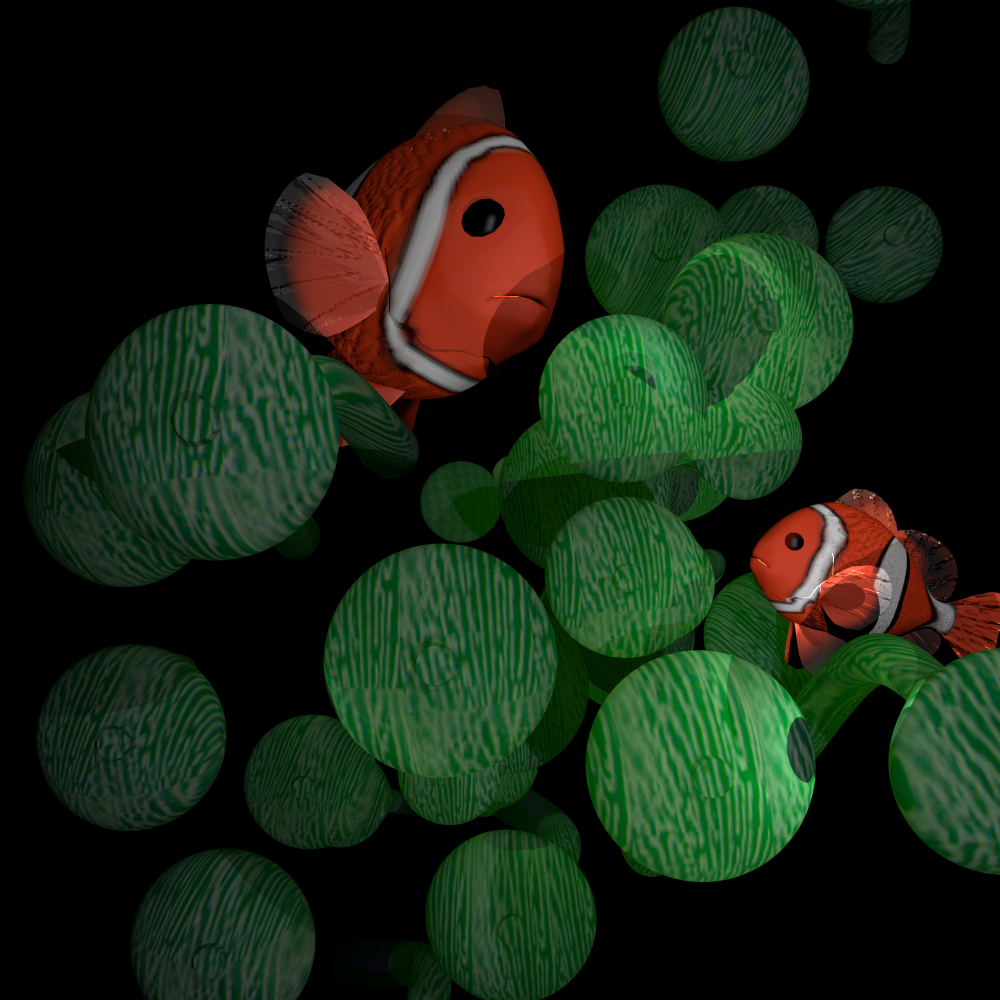
Final Image

A big version of the image can be found here.
Source Code
The new and modified source code files can be found here.
Resources
Pat Hanrahan and Wolfgang Kreuger: "Reflection from Layered Surfaces due to Subsurface Scattering" Computer Graphics (Proc. SIGGRAPH 1993), July 1993
Henrik Wann Jensen, Stephen R. Marschner, Marc Levoy and Pat Hanrahan: "A Practical Model for Subsurface Light Transport". Proceedings of SIGGRAPH'2001.
Henrik Wann Jensen and Juan Buhler: "A Rapid Hierarchical Rendering Technique for Translucent Materials" Proceedings of SIGGRAPH'2002