, it is
considerably more dense than graphs that have been traditionally
regarded as well-suited for tree-based layout methods.
, it is
considerably more dense than graphs that have been traditionally
regarded as well-suited for tree-based layout methods.
The special-purpose MBone and Constellation visualization systems were developed in conjunction with users undertaking a particular focused task. In contrast, the H3 visualization system was not developed using a user-centered design process. It was instead intended as a somewhat more general solution to the problem of scalability in graph layout and drawing systems for an entire class of graphs. In Section 3.1 we define the class of quasi-hierarchical graphs and discuss the kinds of tasks that require viewing them.
Next, in section 3.2, we present a spatial layout algorithm for quasi-hierarchical graphs that uses a spanning tree constructed with the help of domain-specific information as a backbone. The H3 algorithm uses hyperbolic geometry for its computations, so we also present some basic background information about hyperbolic space and its relationship to general distortion-based techniques for visualizing information.
In section 3.3 we present the H3Viewer guaranteed frame rate drawing algorithm, which uses a combination of graph-theoretic and viewpoint information to ensure fluid interaction. Our visual encoding approach is documented in section 3.4, including an analysis of the information density of the H3 approach and the cognitive implications of using a radial layout. Implementation issues, including the desirability of linking the H3Viewer with other views of the dataset, are covered in section 3.5.
Section 3.6 covers interaction. The results of the project are discussed in section 3.7. We begin by documenting that the H3 system can quickly handle datasets more than one hundred times larger than most previous systems, then cover the project outcomes, which include incorporation into a commercial product. We then discuss several additional task domains where people have chosen to use the H3 system, ranging from simply creating data files in the H3 format for quick perusal to creating custom applications using our libraries. Finally, we present the results of a user study that found statistically significant benefits when using the H3Viewer for certain tasks.
Large graphs are extremely difficult to lay out in a way that helps people understand them. In the H3 project our main goal was to push the state of the art in dataset size far past previous limits. We achieved this scalability at the cost of sacrificing generality.
Most traditional taxonomies classify graphs based on purely graph-theoretic properties. For instance, determining whether a graph is acyclic or bipartite is completely independent of the domain of the data. We instead introduce a classification that depends on both graph structure and domain knowledge. We investigated a class of graphs that we call quasi-hierarchical, which can be effectively visualized using a spanning tree as the backbone of a layout algorithm. The visualization challenge is to clearly demarcate the situations in which a tree-based backbone drawing would enlighten rather than mislead the user.
A spanning tree is a connected acyclic subgraph that contains all the vertices of the original graph, but does not have to include all the links. A spanning tree (or a forest of spanning trees) can be computed for any graph. There are many well-known algorithms for building minimum spanning trees from general graphs, such as Kruskal's and Prim's [CLR93, Chapter 24,]. The characterization of building a spanning tree that is most useful for our purposes is to cast it as a problem that must be solved at each node, by selecting which of the incoming links to a node would be the best one to use as the parent for that node in the spanning tree. A slightly more formal definition of a quasi-hierarchical graph is one for which there is a decision procedure for selecting the preferred parent link from among all the incoming links to a node. From a purely graph-theoretic point of view, the problem is simply finding a minimum-weight spanning tree through a graph with weighted edges, where domain-specific information is used to compute the weights.
Trees and directed acyclic graphs (DAGs) are trivially quasi-hierarchical, even without the use of domain knowledge. One might assume at first glance that only graphs that are quite sparse are quasi-hierarchical. For example, a Unix file system is nearly tree-like, since there are relatively few symbolic links. However, graphs that are considerably more dense than trees can also be quasi-hierarchical. The hyperlink structure of the web is a good example, and we discuss it further in the next section. The H3 algorithm can be used on graphs that are not quasi-hierarchical, by simply using a fallback algorithm such as breadth-first search to create a spanning tree, but the resulting visualization will probably not be useful.
Extremely dense graphs are unlikely to be quasi-hierarchical, although
there may be some domains with counterexamples. The examples in this
chapter range from |E| = |V| in the case of trees to |E| = 4|V|
for the Autonomous Systems described in section 3.7.5.
Although even the latter is sparse by
the standard measurements of graph theory, since , it is
considerably more dense than graphs that have been traditionally
regarded as well-suited for tree-based layout methods.
After the core H3 algorithms were developed, we sought task domains where visualizing quasi-hierarchical graphs would be useful. The most important task consideration is whether drawing a graph is at all useful. Many problems could conceivably be cast in graph-theoretic terms, but a visualization is useful only for tasks tied to explicit human understanding of link structure of that graph. If that link structure is indeed relevant and, moreover, there is task domain information available to choose a good parent for each child node, then the H3Viewer is an appropriate visualization tool for the job.
An interactive visual representation of the node-link structure of a graph is helpful when it partially transfers cognitive load to an external representation. We have identified three quite different functions that an external representation can serve for a user:
An example domain where all three of these functions are useful is the creation and maintenance of a large web site, a task where understanding the hyperlink structure of the site is important.
The structure discovery function is relevant because the hyperlink structure of a site has a direct influence on the number of visitors to particular pages: the more clicks it takes a visitor to reach a page from the entry point, the less likely it is to be reached [Nie00]. Site designers usually want to tune sites so that important or popular pages are a minimal number of hops from the root instead of being relegated to obscurity by an overly deep hyperlink structure. The task of organizing a site so that information is categorized in a meaningful and easily traversable way is difficult, in part because it requires keeping track of the relationship of many individual pages and aggregate groups of pages. The size of most nontrivial web sites makes this hard to do without an external representation. For instance, the medium-sized academic web site of the Stanford graphics group has 70,000 pages.
An example of a contextual backdrop is showing traffic log information in the context of the hyperlink structure of the site (see Figure 3.17 in section 3.5.1). A simple ordered list of the most popular pages on a site can be computed from a site's traffic logs and presented to the designer without any need for visualization. However, that list alone is only the beginning of the job. The traffic logs record which outgoing hyperlink is chosen by a visitor to a web page. The designer can often make more informed decisions about site organization if the actual choices made by the visitors are shown in the context of the full range of possibilities -- that is, if the traffic information is presented in relation to the hyperlink structure of the site instead of as a simple list. The graphical representation of the link structure of the site is helpful because it transfers some of the cognitive burden to an external representation, instead of forcing the site designer to reconstruct that structure mentally.
Linking a visualization window to other views gives the webmaster much more flexibility and power than would be possible a single standalone browser. For example, clicking on the node that represents a document in the visualization window would cause it to be rendered in a linked HTML viewer, or typing a search query in another window could trigger an animated transition in the visualization window that ends with the desired node framed in the view. An example is shown in Figure 3.15.
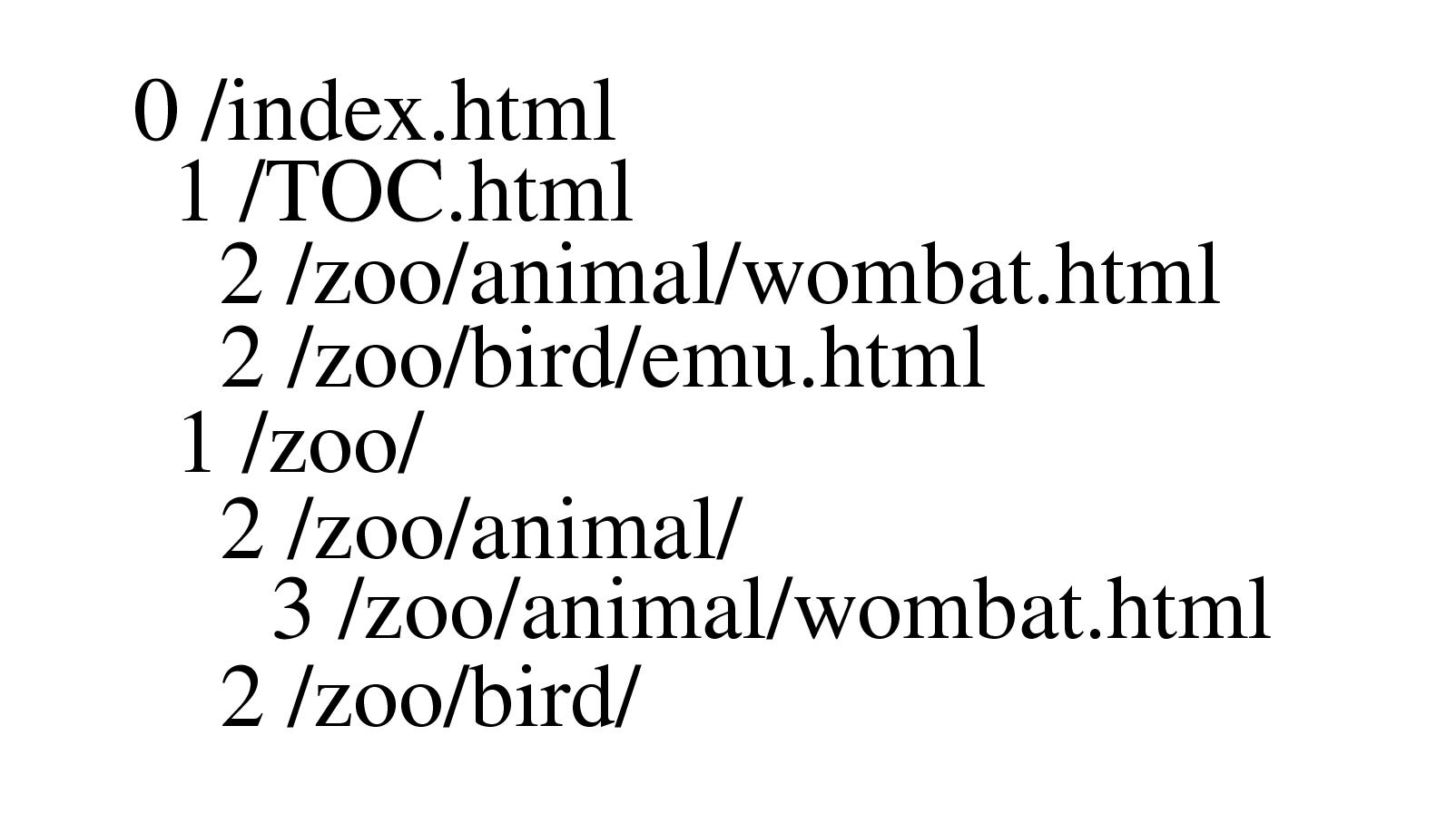


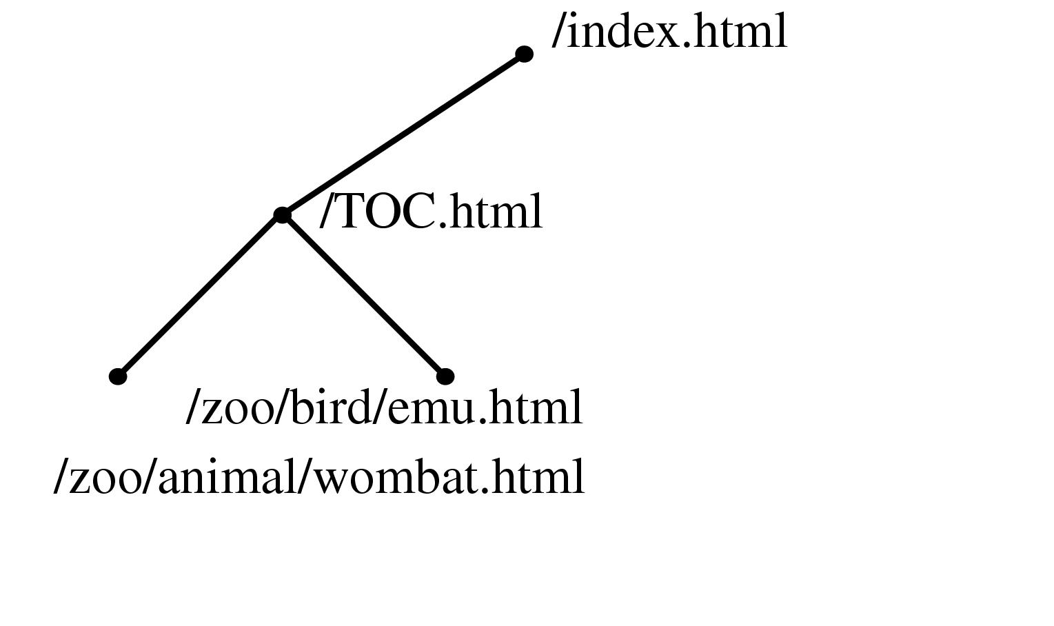

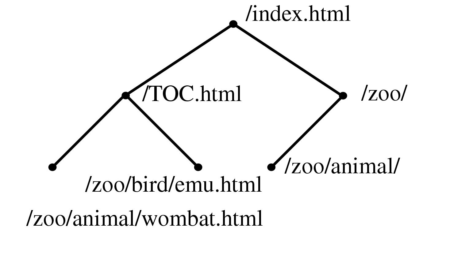
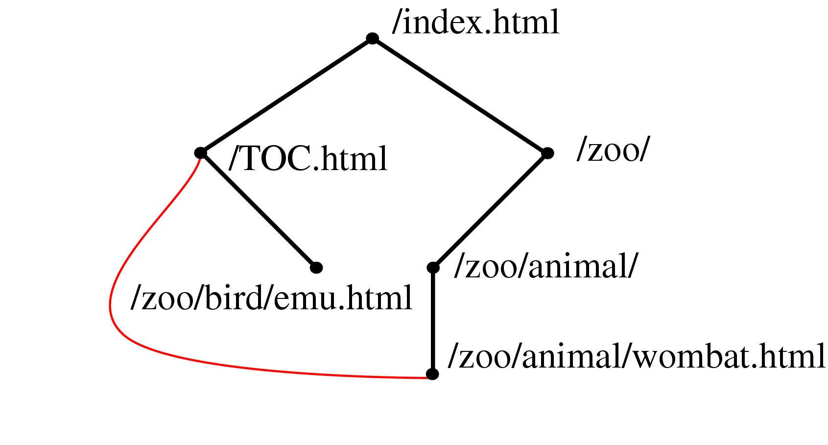

Figure 3.1 Constructing a spanning tree for quasi-hierarchical web site. Top Left: The hyperlink structure of a simple hypothetical site, as it would be reported by a web spider starting at the top page. Nodes represent web pages, and links represent hyperlinks. Although the graph structure itself is determined by hyperlinks, additional information about hierarchical directory structure of the site's files is encoded in the URLs. Top Row: We build up the graph incrementally, one link at a time. Middle Row: We continue adding nodes without moving any of the old ones around. Bottom Row: When the animal/wombat.html page is added, the label matching test shows that animal is a more appropriate parent than /TOC.html, so the node moves and the link between animal/wombat.html and /TOC.html becomes a non-tree link. In the final stage, note that bird/emu.html does not move when the bird is added, even though the labels match, because there is no hyperlink between them.
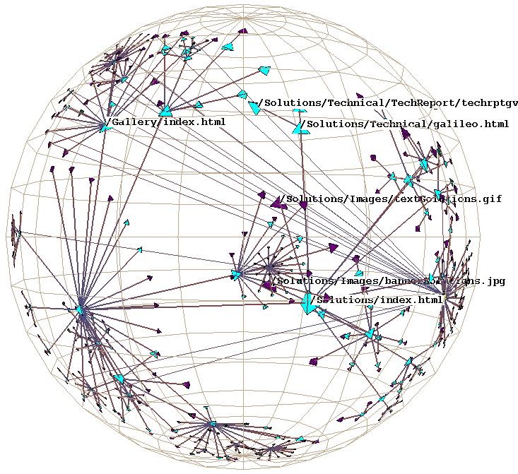
A web site is an example of a quasi-hierarchical graph where nodes represent web documents and the links represent hyperlinks between those documents. Even though web sites are highly interconnected, Web site designers usually have a clear notion of hierarchy within the site: ``Pages within sites are typically organized in hierarchical, tree-like, fashion'' [HA99, p. 2,]. A common mental model for a designer is that most content pages conceptually have a single main parent even though they might have multiple incoming links from related lateral pages. We rely on the pattern that server directories usually have a default document (often called ../index.html#toc) that is a natural parent for every other file in that directory, and that the location of subdirectories is a deliberate choice reflecting the organization of the site content. This heuristic that the directory structure of a web site reflects authorial intent on the part of the site designer is often, but not always, true.
Information about directory structure of a site is easy to obtain, since it is encoded in the URL of the page. We can use this directory information to resolve parentage within the hyperlink graph structure by giving preference to URLs that have as many matching characters as possible from the root on the left towards the right. Figure 3.1.1.2 shows an illustrative example of how a spanning tree would be incrementally formed by parsing a linear file that contains a depth-first traversal of the graph. Nodes are initially directly attached to the first incoming link, but can be moved when a more appropriate match is found. In this case, the label matching has top priority, as shown in the figure. If none of the incoming nodes is a clear choice given the directory structure information, we fall back on a preference for nodes closer to the root so that the resulting spanning tree is closer to breadth-first than depth-first.
When the directory structure of the site does connote authorial intent, then our heuristic is usually a much closer match to the user's mental model than a simple breadth-first layout. For instance, many sites have a table of contents page one hop from the entrance page. Since that page contains a link to every other document at the site, it would end up being the parent of almost every document on the site. The resulting degenerate spanning tree would not encode any interesting structural information.
Although we use the directory structure as a heuristic for making decisions about the spanning tree, the underlying graph that we are laying out is the hyperlink structure of the tree. We are not simply laying out the file system structure of the site: although the nodes are the same in both cases, the links are different.
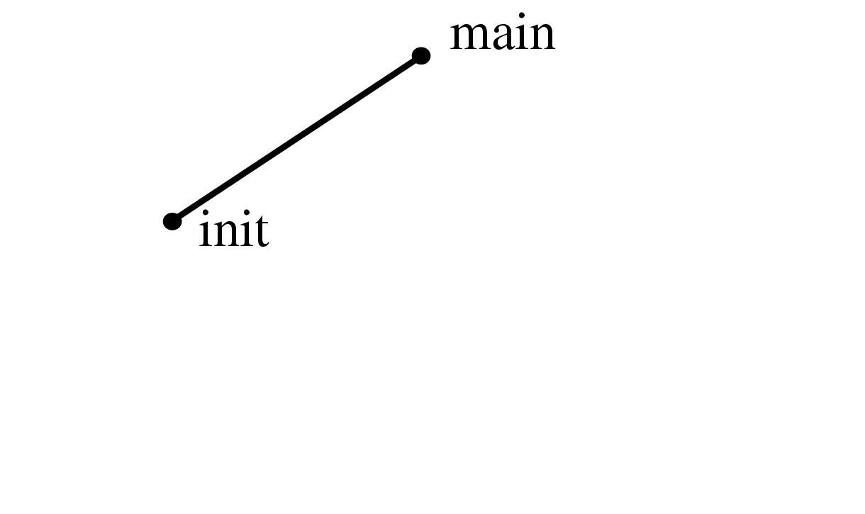


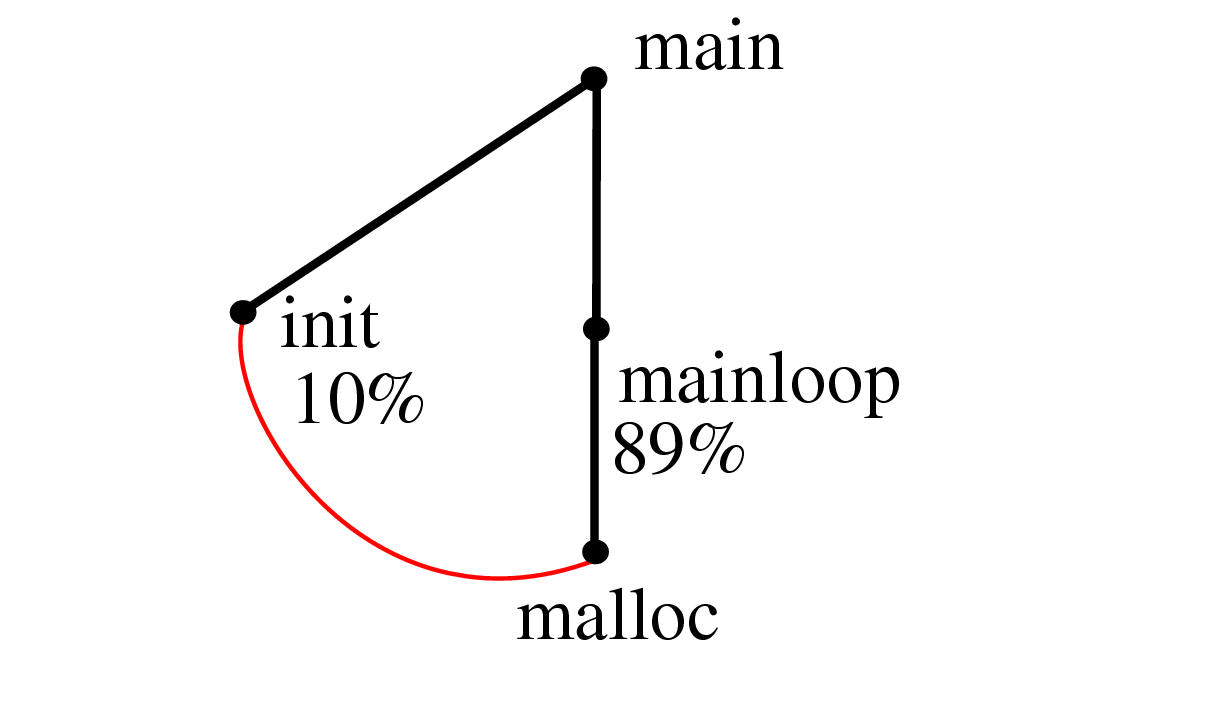
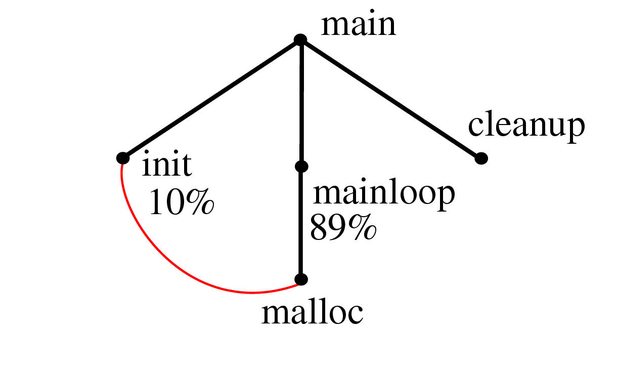
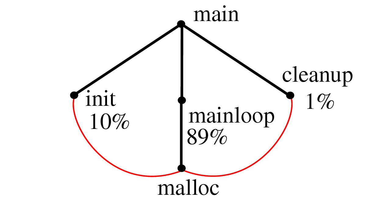
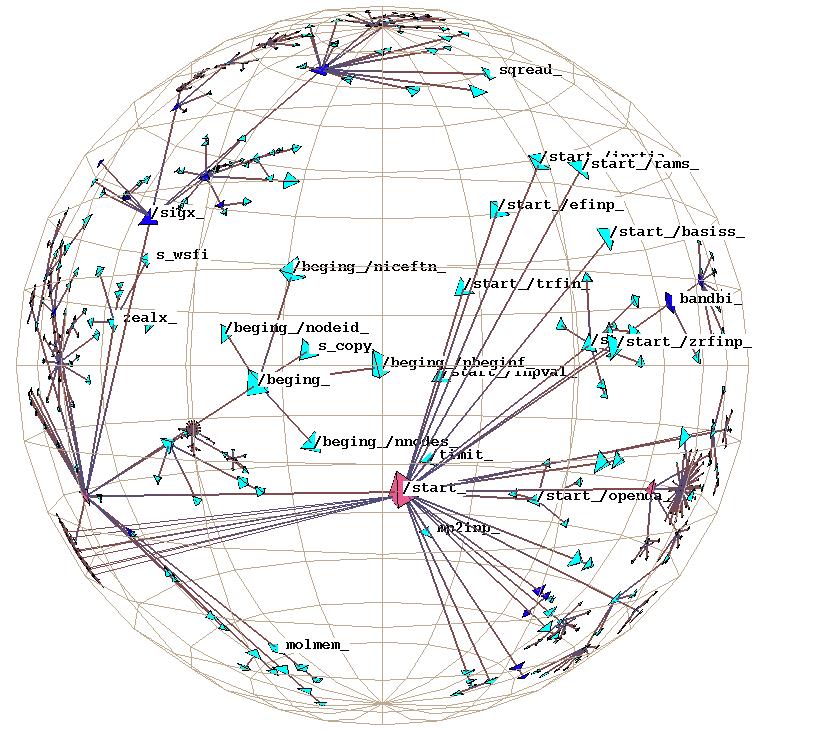
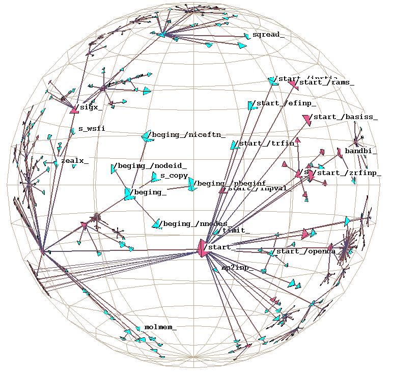
Figure 3.2: Constructing a spanning tree for quasi-hierarchical function call graph. In this simple hypothetical function call graph, nodes represent functions, and links represent calls from one function to another. The call graph is computed by a static analysis of the program text. The spanning tree is determined by run-time profiling of the code so that the calling procedure that is responsible for the most execution time in the called procedure is the parent. We show the layout incrementally as in Figure 3.1.1.2: the parent of a node can change when new information about a more appropriate candidate emerges, and the small multiples should be read row by row starting at the top left.
One task faced by the SUIF compiler research group at Stanford was
optimizing performance by detecting which parts of a program can be
parallelized [HAA 96]. Their methods worked fully automatically up
to a point, but they then relied on user feedback to achieve full
optimization. The SUIF optimizing compiler pinpointed brief
sections of code that were shown to the user. If the user could
assert that certain conditions were met using high-level knowledge not
available to the compiler, then more of the program was successfully
parallelized.
96]. Their methods worked fully automatically up
to a point, but they then relied on user feedback to achieve full
optimization. The SUIF optimizing compiler pinpointed brief
sections of code that were shown to the user. If the user could
assert that certain conditions were met using high-level knowledge not
available to the compiler, then more of the program was successfully
parallelized.
The difficulty faced by the user was understanding how a brief section of code (generally a few lines inside a tight loop) fit into the bigger picture of the entire program. Although an original author might be well aware of the interdependencies, software engineers who were modifying unfamiliar code or authors who had long since forgotten the details of their own code were faced with a challenge. The SUIF developers hoped that an interactive graphical representation of the function call graph would help SUIF users understand a complex program's structure more quickly. Such graphs are notoriously difficult to understand when all the links appear in a 2D nonplanarized layout, which is unfortunately the usual approach even in state-of-the-art performance analysis tools.
In the SUIF graph, nodes represent functions and links represent a call from one function to another. This base graph is known as a static function call graph, where the existence of a call is determined by parsing the program code. The SUIF researchers decided that using execution time measurements to create a spanning tree would result in layouts of these quasi-hierarchical graphs that closely matched their mental model of the structures. They used their existing tools for extracting run-time dynamic profile information to recover the percentage breakdown of the time attributable to each calling procedure out of all the time spent executing the called function. The calling procedure responsible for the majority of a child's execution time was used as the main parent in the spanning tree. Figure 3.2 shows a simple example. (Figures 3.14 and 3.21 show call graphs displayed in our visualization system.)
The previous section covers the motivation for using an appropriate spanning tree as the backbone for the spatial layout of a quasi-hierarchical graph. In this section we discuss how to determine a position in space for each tree node. We first cover the idea of using nonlinear distortion for information visualization, then explain the utility of hyperbolic geometry for distortion-based layout and navigation. We end with the specifics of the H3 hyperbolic tree layout algorithm.
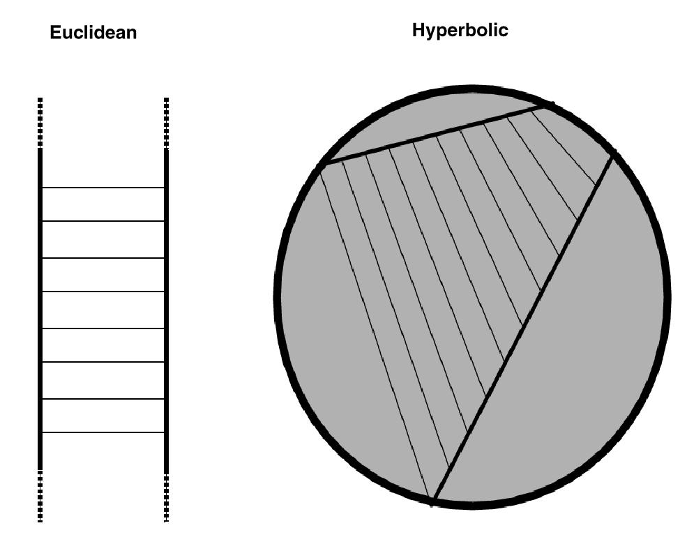
The classic problem with tree layout in Euclidean space is that the number of child nodes to place grows exponentially at each level of the tree, but the available room in which to place them grows only polynomially. Specifically, the circumference of a circle or the area of a sphere increases as a polynomial function of its radius. The usual approach to avoiding collisions is to allocate less room to nodes deeper in the tree than to ones near the root. The disadvantage of this strategy is that only a small local neighborhood of any node can be examined at once because of the size differential between root and leaf nodes. Zooming back to see an overview of the entire tree results in leaf nodes too small to see. Examining nodes deep in the tree requires zooming in so far that surrounding context is lost.
There is a whole class of distortion-based visualization methods that strive to show detail within as much surrounding context as possible in a given amount of screen area, which we discuss in section 2.1. In the H3 system we achieve an elegant single-focus distortion effect by using hyperbolic geometry for both layout and navigation.
Hyperbolic geometry is one of the non-Euclidean geometries developed at the turn of the century. We use it for two reasons: first, there is an elegant way to draw a Focus+Context view using a known projection that maps the entire infinite space into a finite drawing region. Second, we can allocate the same amount of room for each of the nodes in a tree while still avoiding collisions because there is an exponential amount of room available in hyperbolic space.
Hyperbolic and spherical geometry are the only two non-Euclidean
geometries that are homogeneous and have isotropic distance metrics:
in other words, there is a uniform, meaningful, and continuous concept
of the distance between two points.![]() These
geometries are internally consistent despite the lack of Euclid's
parallel postulate. In the spherical case there are no parallel lines:
all great circles intersect each other. (The Planet Multicast system
described in Section 4.2 uses great circles, which
are geodesics on the surface on a 2D sphere, as part of the geographic
layout computation.) In the hyperbolic case there are many lines
through a point that are parallel to another line. The ramifications
of this property are extensive, and it is beyond the scope of this
thesis to discuss their full implications. The following material on
projection and exponential room is only a brief introduction to the
surprising and fascinating mathematics of hyperbolic space, which is
covered in far more detail in many mathematical textbooks
[Mar75,Wol45,Mes64,Cox42,Coo09,Shi63,Ive92,Fen89,Kul61].
These
geometries are internally consistent despite the lack of Euclid's
parallel postulate. In the spherical case there are no parallel lines:
all great circles intersect each other. (The Planet Multicast system
described in Section 4.2 uses great circles, which
are geodesics on the surface on a 2D sphere, as part of the geographic
layout computation.) In the hyperbolic case there are many lines
through a point that are parallel to another line. The ramifications
of this property are extensive, and it is beyond the scope of this
thesis to discuss their full implications. The following material on
projection and exponential room is only a brief introduction to the
surprising and fascinating mathematics of hyperbolic space, which is
covered in far more detail in many mathematical textbooks
[Mar75,Wol45,Mes64,Cox42,Coo09,Shi63,Ive92,Fen89,Kul61].
Figure 3.3: Exponential volume of hyperbolic space. There is literally more room in hyperbolic space than in Euclidean space, as shown in this embedding of the hyperbolic plane into Euclidean 3-space. A circle on a hyperbolic surface has an exponentially increasing circumference, as opposed to the familiar Euclidean situation where circle circumference grows quadratically with respect to its radius. Image from [TW84] used courtesy of Ian Warpole.
In hyperbolic space, circumference and area increase exponentially
with respect to radius. There is literally more room in hyperbolic
space than in Euclidean space, where these measures increase
polynomially.![]()
The circumference of a hyperbolic circle increases exponentially
with respect to its radius; the equation is  , as opposed to the Euclidean
equation
, as opposed to the Euclidean
equation  . Figure 3.3 shows a picture of the 2D
hyperbolic plane embedded into 3D Euclidean space, intended to give an
intuitive sense of how much more room there is on a hyperbolic plane
than on a Euclidean plane. Most pictures of the 2D hyperbolic plane,
for instance Escher-style tilings [Sch92,DLW81], show one of
the traditional projective or conformal views where projected features
appear smaller on the periphery. This picture instead shows a piece of
the 2D hyperbolic plane where true sizes are not distorted, so the
only way to display it in 3D Euclidean space is with overlapping
folds.
. Figure 3.3 shows a picture of the 2D
hyperbolic plane embedded into 3D Euclidean space, intended to give an
intuitive sense of how much more room there is on a hyperbolic plane
than on a Euclidean plane. Most pictures of the 2D hyperbolic plane,
for instance Escher-style tilings [Sch92,DLW81], show one of
the traditional projective or conformal views where projected features
appear smaller on the periphery. This picture instead shows a piece of
the 2D hyperbolic plane where true sizes are not distorted, so the
only way to display it in 3D Euclidean space is with overlapping
folds.
Figure 3.4: Euclidean equidistant parallels vs. hyperbolic divergent parallels. Left: Parallel lines in Euclidean space are always the same distance apart. Right: In hyperbolic space the distance between two lines that never meet does indeed change. Here we show two geodesics that are not equidistant, but extend to infinity without ever intersecting. Recall that the projective model is an open disc, so the boundary is not part of the space.
Considering the distinction between parallel and equidistant lines in hyperbolic space can provide a more focused mathematical intuition for why this holds true. Two parallel straight lines (geodesics) are always the same distance apart in Euclidean space, but in hyperbolic space most parallel straight lines are not equidistant. The two hyperbolic geodesic lines in Figure 3.4 are parallel because they do not intersect, but they are clearly diverging.
Hyperbolic space, like Euclidean space, is infinite in extent. However, it is possible to map the entire infinite space into a finite portion of Euclidean space. That finite projection corresponds to a Euclidean camera taking a picture of an entire hyperbolic universe from the ``outside'', providing a Focus+Context view. Any projection from hyperbolic to Euclidean space will necessarily involve some distortion, since the distance metrics are different. In our case we want to choose the distortion most advantageous for information visualization. Since our goal is a Focus+Context view, we ruled out an ``insider'' projection such as the one used in the pedagogical video Not Knot [GM91,Gun92,PG92]. We want to use a virtual camera that is not constrained by the same rules of hyperbolic motion as the geometric data, so that important information never falls outside of its field of view.
Figure 3.5: Models of hyperbolic space. Left: The projective model
of hyperbolic space, which keeps lines straight but distorts angles.
Right: The conformal model of hyperbolic space, which preserves
angles but maps straight lines to circular arcs. These images were
created with the webviz system from the Geometry Center
[MB95], a first attempt to extend cone tree
layouts to 3D hyperbolic space that had low information density. The
cone angle has been widened to 180 , resulting in flat discs
that are obvious in the projective view. The arcs visible in conformal view
are actually distorted straight lines.
, resulting in flat discs
that are obvious in the projective view. The arcs visible in conformal view
are actually distorted straight lines.
There are several standard projections from hyperbolic to Euclidean space, called models in the mathematical literature. The two that have finite projections are the projective model (sometimes known as Klein, or Klein-Beltrami) and the conformal model (sometimes known as the Poincaré disc or ball). There is a known mapping between these two models, and also between these and the models that have infinite projections, such as the upper half space or Minkowski models. The conformal model preserves Euclidean angle measurements but maps straight lines into arcs. The projective model preserves straight lines but distorts angles. Figure 3.5 shows the different visual appearance of a graph projected projectively and conformally using the webviz system we previously developed at the Geometry Center, which supported both models.
The conformal model is sometimes considered more aesthetically pleasing, at least in two dimensions: the famous Escher pictures of 2D hyperbolic tilings [Sch92,DLW81] are conformal, as is the 2D hyperbolic tree browser developed at Xerox PARC [LRP95]. However, in the 3D case the projective model is much faster for layout and drawing using standard graphics packages.
Most 3D graphics libraries have a highly optimized 4 4 matrix
pipeline, often implemented in hardware, because they use homogeneous
coordinates to efficiently describe transformations of Euclidean
3-space. We can use these standard libraries for efficient computation
of our hyperbolic transformations in the projective model, since they
can conveniently also be encoded as 4
4 matrix
pipeline, often implemented in hardware, because they use homogeneous
coordinates to efficiently describe transformations of Euclidean
3-space. We can use these standard libraries for efficient computation
of our hyperbolic transformations in the projective model, since they
can conveniently also be encoded as 4 4 matrices. In contrast,
transformations in the conformal model require 2
4 matrices. In contrast,
transformations in the conformal model require 2 2 complex
matrices, which cannot be trivially transformed into a more standard
operation. Moreover, standard graphics libraries are much slower when
drawing curved objects than flat ones, since curves are approximated
by many piecewise linear lines or polygons. Since the main goal of the
H3 system was scalability to large datasets, we chose to use the
projective model. An extensive discussion of 3D hyperbolic projective
transformations for use in computer graphics appears in a paper by
Phillips and Gunn
[PG92], so we do not discuss these in detail here.
2 complex
matrices, which cannot be trivially transformed into a more standard
operation. Moreover, standard graphics libraries are much slower when
drawing curved objects than flat ones, since curves are approximated
by many piecewise linear lines or polygons. Since the main goal of the
H3 system was scalability to large datasets, we chose to use the
projective model. An extensive discussion of 3D hyperbolic projective
transformations for use in computer graphics appears in a paper by
Phillips and Gunn
[PG92], so we do not discuss these in detail here.
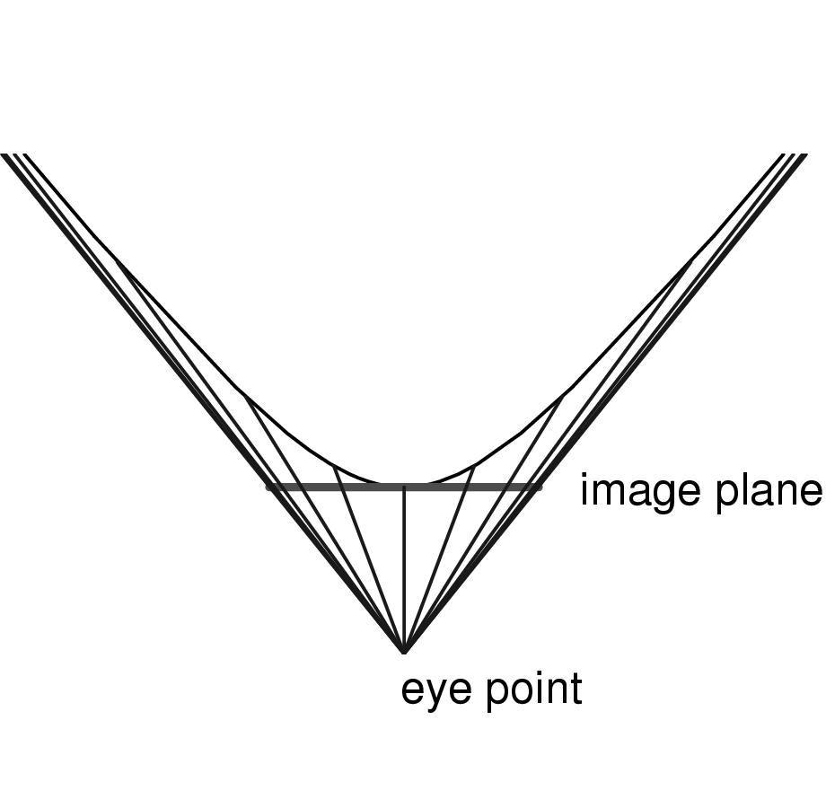
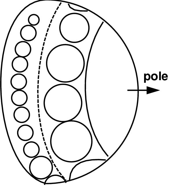
Figure 3.6: 1D hyperbolic projection. An illustration of the projective model for one-dimensional hyperbolic space. The image plane is at the pole of one sheet of the hyperbola and the eye point is where the asymptotes meet. Although the projection near the pole is almost undistorted, the apparent shrinkage increases as the rays reach further up the hyperbola.
The procedure for projecting from hyperbolic to Euclidean space under the Klein-Beltrami model is easiest to understand by first looking at the one-dimensional case shown in Figure 3.6. The entire hyperbola can be projected onto a finite Euclidean open line segment tangent to its pole, using an eye point one unit below that pole. The asymptotes of the hyperbola are the boundaries of the line segment and cross at the eye point. Objects (in this case, 1D lines) drawn on the hyperbola itself can be projected to the line segment. The projections of objects exactly at the pole are undistorted, but objects far from the pole project to a vanishingly small part of the line segment. Rigid hyperbolic objects that translate along the hyperbola will appear in the projection to grow to a maximum when at the pole and then shrink, and after translating infinitely up the hyperbola their projection will be infinitely close to the line segment border.
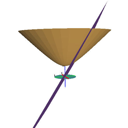
Figure 3.7: 2D hyperbolic projection. An illustration of the projection from a unit hyperboloid to a Euclidean disc at z=0. Left: A cutting plane which goes through the origin is shown nearly edge-on: it intersects the hyperboloid in a geodesic, and the disc in a straight line. Right: We show the same scene from a different angle, so that the purple cutting plane is nearly parallel to the image plane.
Figure 3.7 shows the two-dimensional case: the surface of the hyperboloid projects into a disc -- a finite section of a Euclidean plane. The plane is arranged so that it cuts the hyperboloid in a geodesic line, which projects to a straight line in the disc at z=0. Hyperbolic translation amounts to sliding 2D objects around on the hyperbola itself. Again, the size of the projected objects depends on their proximity to the pole, which projects to the origin of the disc.
The 3D case is hard to show in a diagram, since it involves a
3-hyperboloid projected into a ball -- a finite section of Euclidean
3-space. The pole of the hyperboloid projects to the origin of the
ball. In the previous figures we chose to diagram objects of dimension
n embedded in a space of dimension n+1 only for clarity of
exposition.![]() Although Figure 3.7 shows the
2-hyperboloid embedded in 3D space, projecting from it to the disc is
a purely two-dimensional operation. Likewise, although drawing a
diagram for the 3D case would require embedding these 3D objects in
4-space
Although Figure 3.7 shows the
2-hyperboloid embedded in 3D space, projecting from it to the disc is
a purely two-dimensional operation. Likewise, although drawing a
diagram for the 3D case would require embedding these 3D objects in
4-space![]() , the actual mathematics involved is purely
three-dimensional.
, the actual mathematics involved is purely
three-dimensional.![]()
With a single still image, a projection from hyperbolic space looks similar to a Euclidean scene projected through a fisheye lens. The projection to hyperbolic space serves the purpose of a Degree of Interest function as required by Furnas [Fur86]. However, motion of an object constructed with hyperbolic geometry is qualitatively different from the motion of a Euclidean object. Although we could simply place Euclidean objects into hyperbolic 3-space and move them around according to the rules of hyperbolic geometry, we would not be exploiting the exponential amount of room available in hyperbolic space.
The exponential amount of room in hyperbolic space is an elegant ``impedance match'' for a tree layout, since the number of nodes in a tree grows exponentially with its depth. To the best of our knowledge, the idea of using hyperbolic space for tree layout was first informally proposed by Thurston at least as early as the 1980's. Visualization systems for doing so were created independently and nearly simultaneously by both Lamping, Rao, and Pirolli at Xerox PARC [LR94,LRP95], and pre-dissertation work by myself and Paul Burchard at the Geometry Center [MB95].
In Euclidean space, trees can be laid out compactly only if the amount of space devoted to each node grows smaller towards the leaves. When inspecting detail at the leaf level, the structure near the root is difficult to understand because of the major differences in scale. Nodes can be allocated equal size only for a layout that is very sparse, which makes comparisons between levels equally difficult.
However, we can draw a tree in hyperbolic space compactly while allocating the same amount of hyperbolic space for each leaf node no matter how deep it is in the tree. The root node is then the same size as any other node and is special only in that it has no parent. The entire tree structure has roughly equal local information density. Setting the focus for the visualization is simply a matter of translation on the 3-hyperboloid to bring the desired node to the pole. Its projection at the origin of the ball will be large, and many of the nearby nodes will be visible for additional context.
The H3 algorithm can be thought of as an extension of the influential
Cone Tree system developed at Xerox PARC [RMC91]. The Cone
Tree algorithm lays out tree nodes hierarchically in 3D Euclidean
space, with child nodes placed on the circumference of a cone
emanating from the parent. The webviz project at the Geometry
Center [MB95] was a first attempt to adapt the Cone Tree
algorithm for use in 3D hyperbolic space. The webviz layout, shown in
Figure
3.5, used a cone angle of  , widening
the cone into a flat disc. That algorithm did exploit some of the
exotic properties of 3D hyperbolic space, but did not unleash its full
potential: the amount of displayed information compared to the amount
of white space was quite sparse.
, widening
the cone into a flat disc. That algorithm did exploit some of the
exotic properties of 3D hyperbolic space, but did not unleash its full
potential: the amount of displayed information compared to the amount
of white space was quite sparse.
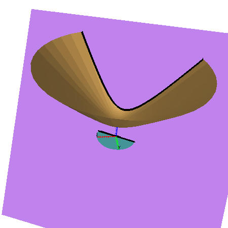
Figure 3.8: Circumference vs. hemisphere. The H3 layout on the surface of a spherical cap at the mouth of a cone is much more compact than the traditional cone tree layout on the circumference of the cone mouth. All three pictures show 54 child nodes in hyperbolic space. Left: The traditional perimeter layout requires a large cone radius, such that it is quite sparse. Middle: The hemispherical layout is scaled so that the child node sizes and cone radius can be directly compared with the perimeter image on the left. Right: The hemispherical layout is scaled so that the parent node size can be directly compared with the perimeter image on the left.
Our H3 algorithm instead lays out child nodes on the surface of a
hemisphere that covers the mouth of a cone, like sprinkles on an ice
cream cone. Figure 3.8 compares this layout to the
original cone tree approach. Like the webviz algorithm, we use a cone angle of
180 to subtend an entire hemisphere. The cone body proper no
longer takes up space but flattens out into a disc at the base of the
hemisphere. The child hemispheres lie directly on the parental
hemisphere's tangent plane, with no visible intervening cone body.
Our hemispherical layout is both possible and effective because of the
exponential amount of room in hyperbolic space.
Specifically, the surface area of a hemisphere,
to subtend an entire hemisphere. The cone body proper no
longer takes up space but flattens out into a disc at the base of the
hemisphere. The child hemispheres lie directly on the parental
hemisphere's tangent plane, with no visible intervening cone body.
Our hemispherical layout is both possible and effective because of the
exponential amount of room in hyperbolic space.
Specifically, the surface area of a hemisphere,  ,
increases polynomially with respect to its radius in Euclidean space.
In hyperbolic space the formula for hemisphere area is
,
increases polynomially with respect to its radius in Euclidean space.
In hyperbolic space the formula for hemisphere area is  , and the hyperbolic sine and cosine functions (
 and
and
 ) are exponential.
The layout algorithm requires two passes: a bottom-up pass to estimate the radius needed for each hemisphere to accommodate all its children, and a top-down pass to place each child node on its parental hemisphere's surface. These steps cannot be combined because we need the radius of the parental hemisphere before we can compute the final position of the children.
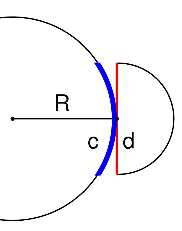
Figure 3.9: Discs vs. spherical caps. The area of a disc underneath a child hemisphere is an approximation for the area of the underlying spherical cap on the parent. This figure shows the 2D case, where the diameter d underneath the half-circle approximates the arc c. The approximation, which works well when there are many children, is necessary because the spherical cap area is not computable without the parental radius R.
We draw leaf nodes as tetrahedra of a fixed hyperbolic size; therefore, we trivially know the value of the radius of child hemispheres at the leaves. At each level we need to determine how large of a hemisphere to allocate for a parent hemisphere given the radii of all the child hemispheres. We do this by summing the area of the disc at the bottom of each child hemisphere.
The flat disc at the bottom of a child hemisphere is only an approximation of the area that will be used when the child is placed on the parental hemisphere. Figure 3.9 shows that the correct area would be the spherical cap that lies underneath the child hemisphere when it covers part of the parental hemisphere, as opposed to a flat disc on the tangent plane. However, computing the area of that spherical cap requires knowledge about the radius of the parental hemisphere, which we do not know since that is exactly what we are trying to discover. The area of the flat disc is a reasonable approximation when the child hemisphere subtends a small angle; that is, when a parent has many child nodes. The approximation breaks down when the number of children is small, but the special cases for properly handling a small number of children (1, 2, or 3 through 5) are easy to handle in the code.
The bottom-up estimation pass starts at the leaves and ends with an estimate of the radius of the root hemisphere. We then use these radius estimates in the top-down pass to compute the actual point in space so as to place child hemispheres on the surface of their parent.
The problem of placing circles contiguously without overlaps has received extensive attention from mathematicians, under the name circle packing or sphere packing [CS88]. A related problem is that of distributing points evenly on a sphere [SK97]. Our particular instance is that of packing circles (1-spheres) on the surface of an ordinary sphere (2-sphere).
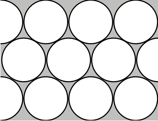
Figure 3.10: Circle packing. Packing uniformly sized circles on a plane is one of the most common circle packing cases. Note that even in this optimal packing of circles on the plane, the area of the circles sums to less than the area of the underlying plane, because of the grey interstitial gaps.
The particular requirements of our situation are somewhat different than the usual cases addressed in the literature, such as packing circles on a 2D plane as in Figure 3.10. Our circles are of variable size, and we are interested in a hemisphere as opposed to a sphere. More importantly, our solution must be fast and repeatable. Our solution cannot involve randomness: given the same input, we must generate the same output. We care far more about speed than precision. An approximate layout is fine for our purposes, whereas a perfect but slow iterative solution would be inappropriate.
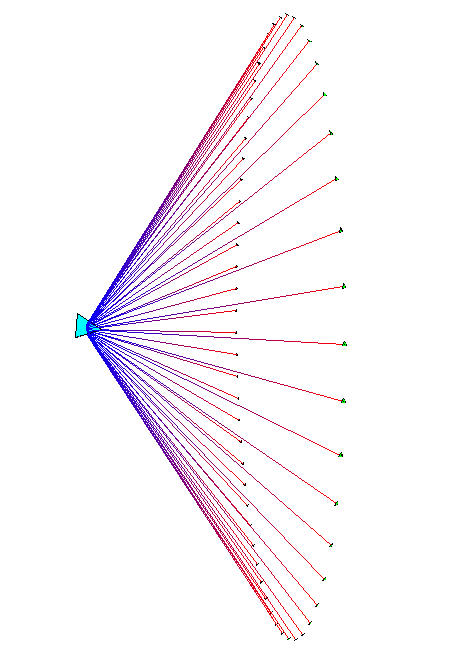
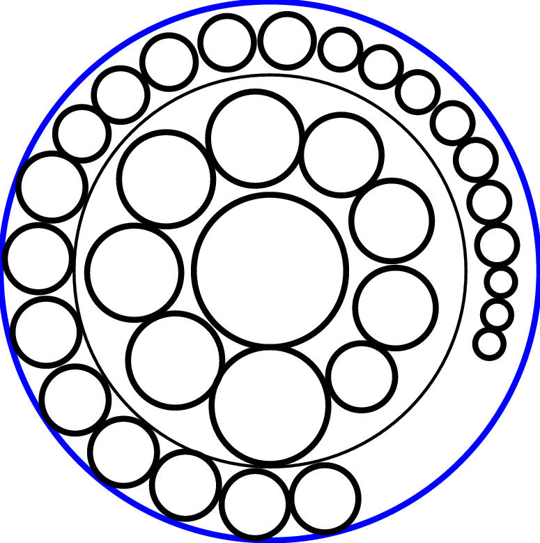
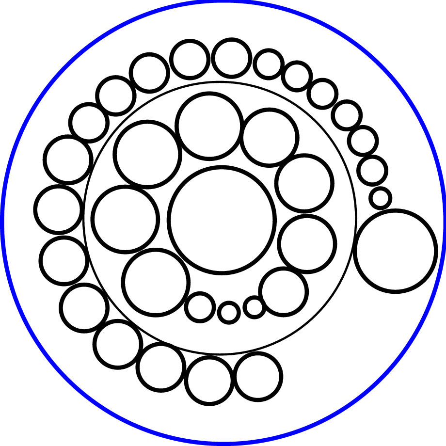
Figure 3.11: Band layout. Left: Discs at the bottom of child hemispheres are laid out in bands on the parent in sorted order according to the number of their descendants, with the most prolific at the pole. Middle: Sorting the children by total progeny results in a list of hemispheres sorted by radius size. Right: Unsorted hemispheres potentially result in a large amount of wasted space within the bands.
Our solution is to lay out the discs in concentric bands centered along the pole normal to the sphere at infinity. The left side of Figure 3.11 shows a view of a parent hemisphere from the side, with only the footprints of the child hemispheres drawn. We sort the child discs by the size of their hemispheres. This number, which is recursively calculated in the first bottom-up pass, depends on the total number of their descendants, not just their first-generation children. The ones that require the most area (i.e. the ones with the most progeny) are closest to this pole. The middle and right of Figure 3.11 compare the amount of space used by this sorted packing with the amount potentially wasted by an unordered packing. The equatorial (bottom-most) band is usually only partially complete.
Even if our circle packing were optimal, the area of the hemisphere required to accommodate the circles would be less than than the sum of the spherical caps subtended by those circles, since we do not take into account the uncovered gaps between the circles (as shown in Figure 3.9). Moreover, our banding scheme is easy to implement but is far from an optimal circle packing. We waste the leftover space in the equatorial band, which in the worst case contains only a single disc. If we did not sort the child discs by size the discrepancy would be even greater, in the worst cases by a factor of 2.
In summary, our estimated target surface area is only an approximation for three reasons. First, the surface area of a spherical cap is greater than the area of a flat disc on a tangent plane to the sphere. Second, even an optimal circle packing leaves uncovered gaps between the discs. Third, our circle packing is known to be suboptimal: circles may use less vertical space than their allotted band allows, and the packing may allow unused horizontal space in the outermost band.
All three reasons lead to an estimate that is less than the necessary area. We use an empirically derived area-scaling factor to increase the radius by an amount proportional to the estimate. In rare cases our initial adjusted estimate of the hemisphere area falls short, when at the end of the placement pass for a hemisphere we find that the incrementally placed child discs extend beyond the allocated hemisphere into the other half of the sphere. We then run a second iteration for placement using the exact size needed for the parental hemisphere radius, which is now directly computable.
The radius estimate scaling factor is one of the two parameters that controls the density of the layout. The other parameter in our implementation is the surface area allotted for hemispheres of leaf nodes. The layout would be too dense if the leaf nodes touch, so we generally specify a larger area than a hemisphere that would exactly fit around the geometric representation of a node.
The H3 layout method operates in two passes. In the bottom-up pass we
find an approximate radius for each hemisphere, and in the top-down
pass we place children on the surface of their parent hemisphere. Here
we present a detailed derivation of the radius  of a parental
hemisphere and the spherical coordinate triple
of a parental
hemisphere and the spherical coordinate triple  needed to place a child hemisphere on the surface of that
parental hemisphere. For each step of the derivation, we show first
the Euclidean then the hyperbolic result. The Euclidean and hyperbolic
formulas used are collected in Table 3.1.
needed to place a child hemisphere on the surface of that
parental hemisphere. For each step of the derivation, we show first
the Euclidean then the hyperbolic result. The Euclidean and hyperbolic
formulas used are collected in Table 3.1.
Table 3.1: Euclidean and hyperbolic formulas.
We compute a target surface area  of a
hemisphere at level p by summing the areas of the discs at the
bottom of the child hemispheres at level p+1.
The Euclidean derivation is straightforward. The Euclidean hemisphere
area formula is
of a
hemisphere at level p by summing the areas of the discs at the
bottom of the child hemispheres at level p+1.
The Euclidean derivation is straightforward. The Euclidean hemisphere
area formula is  , so the Euclidean radius
  would be
  . The area of a Euclidean circle is
  , so the relationship between the parent and child hemispheres is

where  is the area of a disc at the bottom of a child
hemisphere at level p+1 and n is the number of children at that
level.
When we use the hyperbolic hemisphere area formula
is the area of a disc at the bottom of a child
hemisphere at level p+1 and n is the number of children at that
level.
When we use the hyperbolic hemisphere area formula  , the hyperbolic radius of the parental hemisphere is
  . The hyperbolic circle area
formula is considerably different from the Euclidean case:
. The hyperbolic circle area
formula is considerably different from the Euclidean case:  . The parent-child relationship becomes

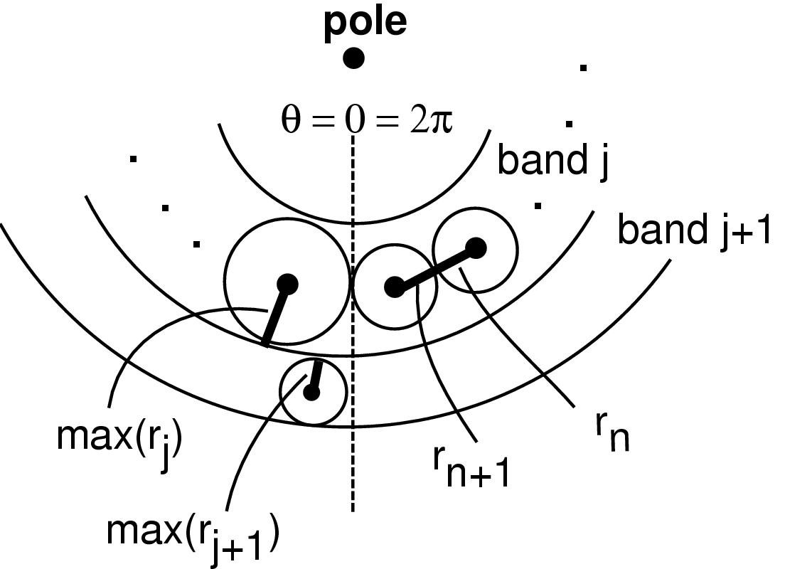
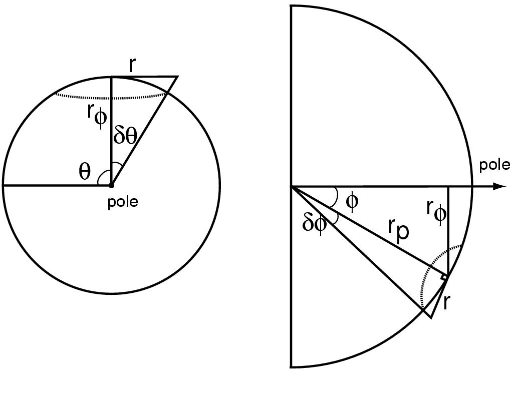
Figure 3.12: Child hemisphere
placement. Left: Within a band, we increment  to move
from the center of one child with radius
to move
from the center of one child with radius  to the center of the
next with radius
to the center of the
next with radius  . When band j is filled at
  , we increment
  to move to a new band j+1 further away from the
pole. The sorting guarantees that first child placed has maximum
radius in the band. Middle: View from above the pole shows the
trigonometry needed to find the incremental
to move to a new band j+1 further away from the
pole. The sorting guarantees that first child placed has maximum
radius in the band. Middle: View from above the pole shows the
trigonometry needed to find the incremental  to move
within a band.
to move
within a band.  is the radius of a spherical cap at
  .
Right: View from the side shows finding the incremental
.
Right: View from the side shows finding the incremental
 to move between bands. The radius of the parent
hemisphere is
to move between bands. The radius of the parent
hemisphere is  .
.
 of the parent
hemisphere to compute the remaining two spherical coordinates
of the parent
hemisphere to compute the remaining two spherical coordinates  and
and  , since the triple
  completely
specifies the position of the child hemisphere at level p+1. We
compute
completely
specifies the position of the child hemisphere at level p+1. We
compute  and
and  cumulatively, starting from the pole at
the top of the hemisphere. The children are laid out in bands that are
concentric around the pole. The band at the pole itself is the
degenerate case of a spherical cap, therefore no value of
cumulatively, starting from the pole at
the top of the hemisphere. The children are laid out in bands that are
concentric around the pole. The band at the pole itself is the
degenerate case of a spherical cap, therefore no value of  needs to
be computed. The total incremental angle
needs to
be computed. The total incremental angle  between child n and child n+1 on a typical band j is the sum of
the angles
between child n and child n+1 on a typical band j is the sum of
the angles  and
and  , which depend on
the radii
, which depend on
the radii  and
and  of the children, as shown in Figure
3.12 on the left. We thus need to derive the angle
of the children, as shown in Figure
3.12 on the left. We thus need to derive the angle
 given some r, as in the middle of Figure
3.12. That angle depends on
given some r, as in the middle of Figure
3.12. That angle depends on  , the radius of
the spherical cap at
, the radius of
the spherical cap at  . We can use a Euclidean right triangle
formula to find the radius
. We can use a Euclidean right triangle
formula to find the radius  , and with the
other Euclidean right-angle triangle formula
, and with the
other Euclidean right-angle triangle formula  we find the Euclidean angle

If we instead use the
hyperbolic right triangle formula to find the radius  and the other hyperbolic right-angle triangle
formula
and the other hyperbolic right-angle triangle
formula  ,
we find the hyperbolic angle
,
we find the hyperbolic angle

We substitute  and
and  to obtain our total incremental
angle for placing a circle within a band:
to obtain our total incremental
angle for placing a circle within a band:

If the total cumulative angle  is
greater than
is
greater than  , we drop down to the next band j+1 and reset
 to 0.
The
to 0.
The  angle between a child on one band and a child on the
next band depends on the radius
angle between a child on one band and a child on the
next band depends on the radius  of the largest child in band j
and the radius
of the largest child in band j
and the radius  of the largest child in band j+1. In our
current circle packing approach, we know that the first child in each
band will have the largest radius, since we lay out the children in
descending sorted order.
We thus need to derive the angle
of the largest child in band j+1. In our
current circle packing approach, we know that the first child in each
band will have the largest radius, since we lay out the children in
descending sorted order.
We thus need to derive the angle  given some r, as in
the right of Figure 3.12. The Euclidean angle
given some r, as in
the right of Figure 3.12. The Euclidean angle  corresponding to r is simply
  because of the
right angle formula. We substitute the hyperbolic formula for
right-angle triangles to find
because of the
right angle formula. We substitute the hyperbolic formula for
right-angle triangles to find

We substitute  and
and  to obtain our total incremental
angle for placing a circle on the next band:
to obtain our total incremental
angle for placing a circle on the next band:

Armed with the triple  , we can center the child
hemisphere in the appropriate spot on the parent hemisphere.
We discuss the tradeoffs of our layout technique further in section
6.1.3 (page
, we can center the child
hemisphere in the appropriate spot on the parent hemisphere.
We discuss the tradeoffs of our layout technique further in section
6.1.3 (page ![]() ).
).
Although we have discussed our algorithm in terms of a bottom-up pass followed by a top-down pass for expository purposes, the necessary work can be done with single recursive function. The recursion starts with the root node, and the base cases are the leaf nodes of known radius. The function begins by looping through the children and calling the layout function recursively on each. Popping the stack after the recursive call yields the child radius, which we can use to compute the parental hemisphere radius estimate, and then immediately place the child discs on the surface of the parent.
Our adaptive drawing algorithm is linear in the number of visible nodes and edges. The projection from hyperbolic to Euclidean space guarantees that nodes sufficiently far from the center will project to less than a single pixel. Although there are a potentially unlimited total number of nodes and edges, our algorithm terminates when features project to subpixel areas. Thus the visual and computational complexity of the scene has guaranteed bound -- only a local neighborhood of nodes in the graph will be drawn.
A guaranteed frame rate is extremely important for a fluid interactive user experience. The H3Viewer adaptive drawing algorithm is designed to always maintain a target frame rate even on low-end graphics systems. A high frame rate is maintained by drawing only as much of the neighborhood around a center point as is possible in the allotted time.
The drawing algorithm incorporates knowledge of both the graph structure and the current viewing position. We use the link structure of the spanning tree to guide additions to a pool of candidate nodes and the projected screen area of the nodes to sort the candidates.
The link structure of the spanning tree provides us with a graph-theoretic measure of the distance between two nodes: the number of hops from one node to another is the integer number of links between them. When we draw a node, reasonable candidates for drawing next are the nodes one hop away, namely its parent and children in the spanning tree. Nodes that are a short number of hops from the center will usually be more visible than those that are a large number of hops away. However, if we simply rely on graph structure, we may waste time filling in sections that are less visible while neglecting those that are more prominent. Although the hop count between two nodes does not change during navigation, the projected screen area of a node depends on the current position of the graph in hyperbolic space. Navigation occurs by moving the object in hyperbolic space, which is always projected into the same fixed area of Euclidean space. Motion on the surface of the 3-hyperboloid brings some node of the graph closest to the pole, such that its projection into the ball is both closest to the origin and largest. Most previous systems for adaptive drawing [Hop97] state the viewpoint problem in terms of camera location, but for convenience in our case we consider instead the mathematically equivalent problem of an object position with respect to a fixed camera.
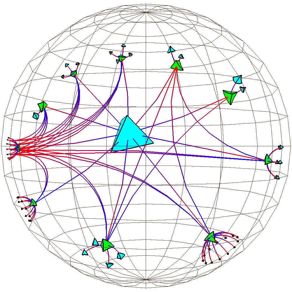
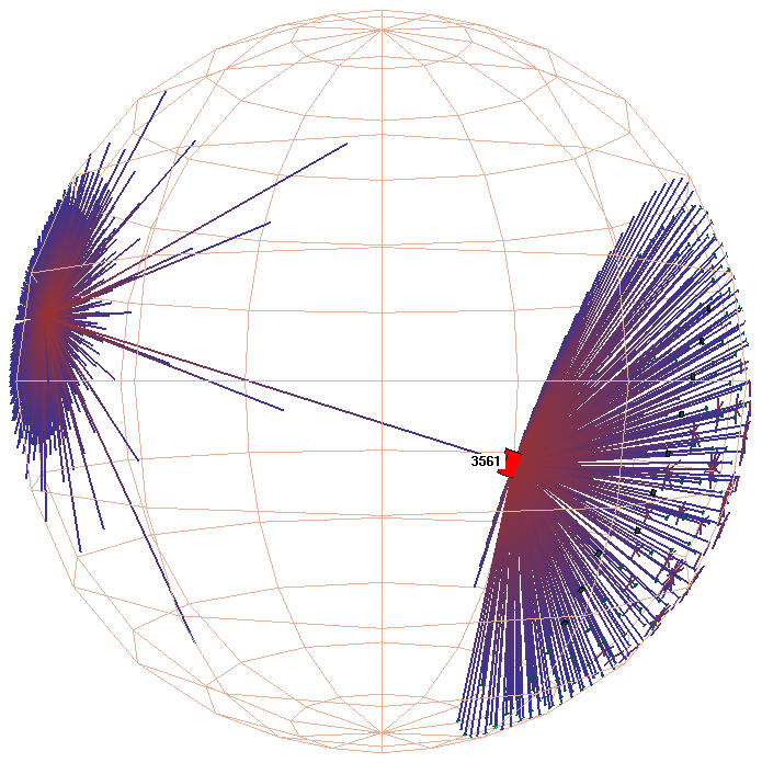
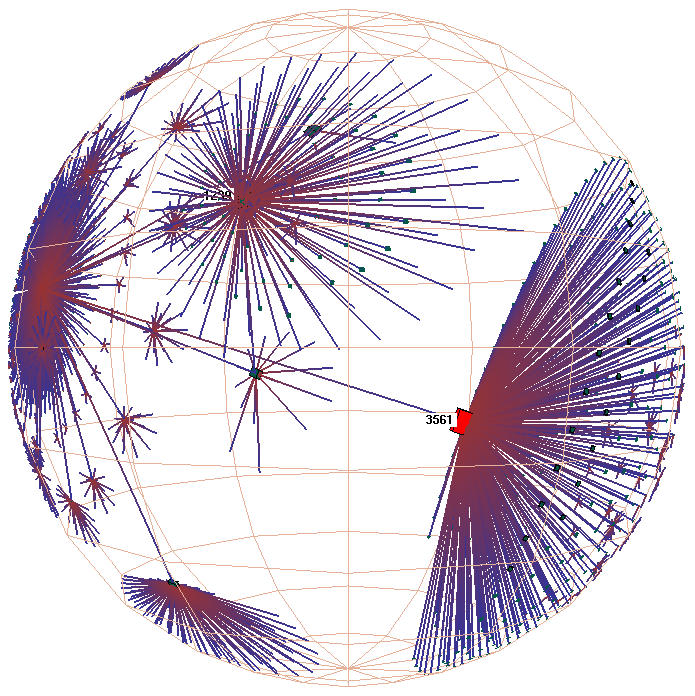
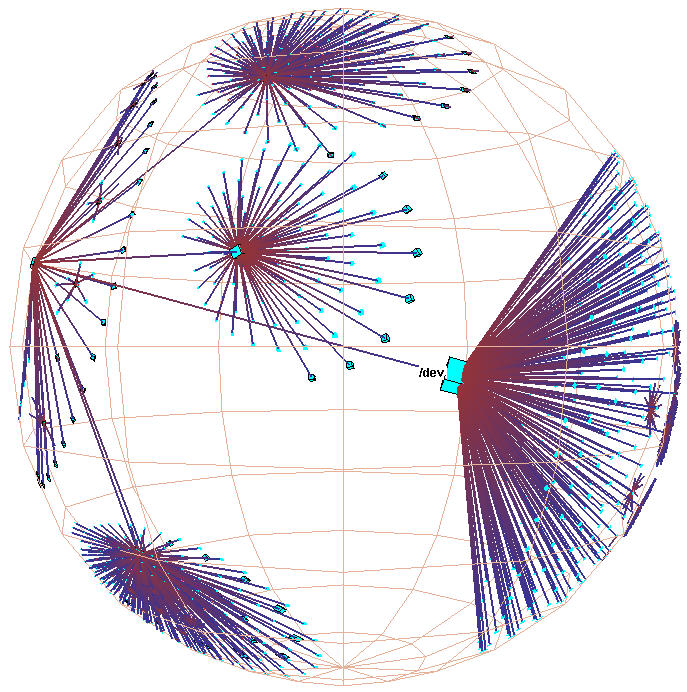
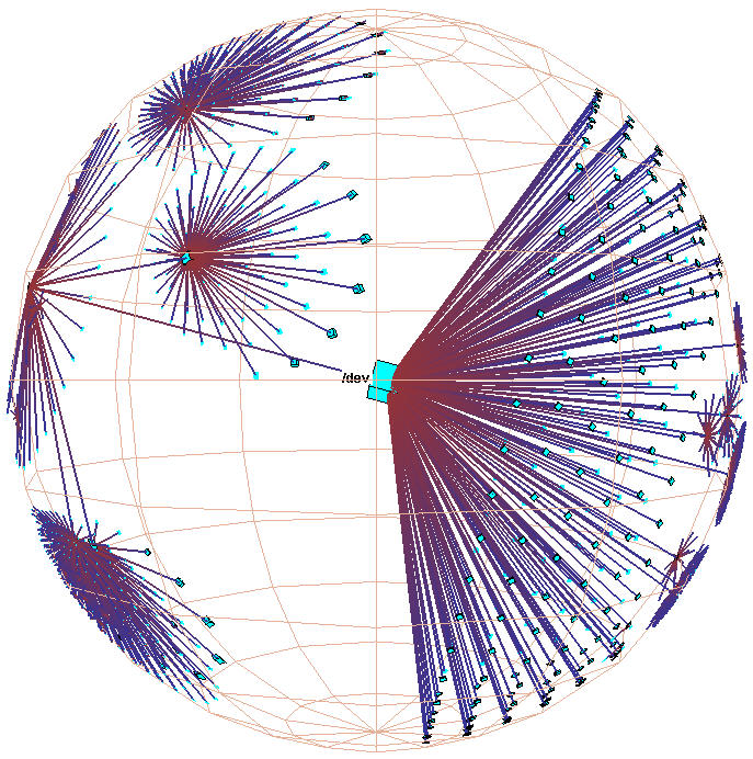
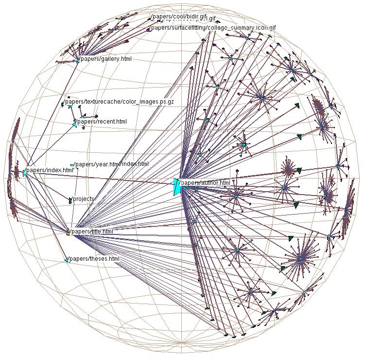
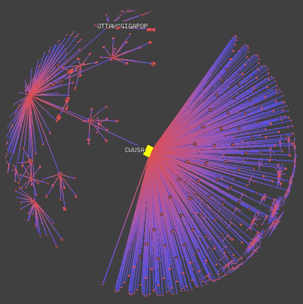
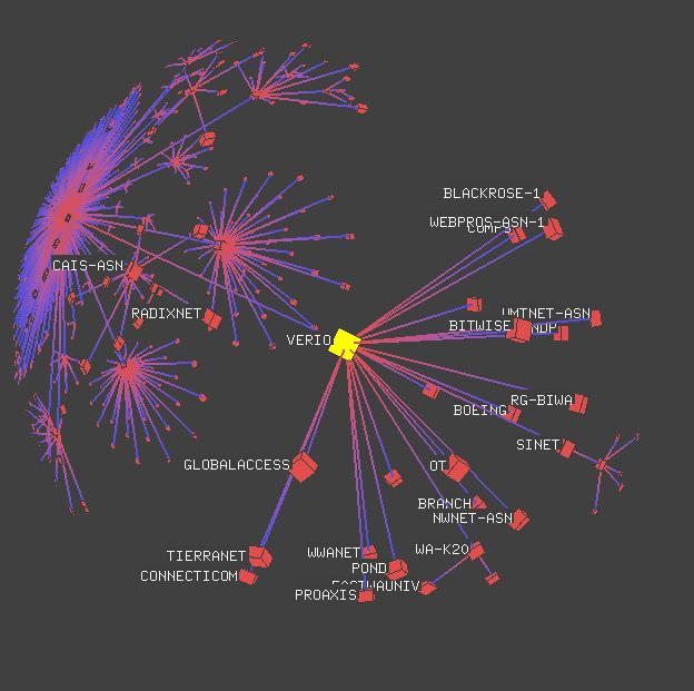
Figure 3.13: Active vs. idle frames, obvious case.
The H3Viewer guaranteed frame rate mechanism ensures
interactive response for large graphs, even on slow machines. Left:
A frame drawn in 1/20th of a second during user interaction.
Right: A frame filled in by the idle callbacks
for a total of 2 seconds after user activity stopped. The graph shows
the peering relationships between Autonomous
Systems, which constitute the backbone of the Internet.![]() The 3000 routers
shown here are connected by over 10,000 edges in the full graph.
The 3000 routers
shown here are connected by over 10,000 edges in the full graph.
also shows that we deliberately draw all links into and out of a node, even if we do not have time to draw the node at the other end. The presence of an unterminated link during motion hints to the user of something interesting in that direction. This situation occurs frequently when drawing nontree links, whose other end often lies far enough away from the center that the drawing loop ends before the terminating node can be drawn.
Our drawing algorithm is built around two queues: the ActionQueue and the DrawnQueue, both of which contain nodes that are kept sorted by projected screen area. These queues are manipulated differently based on the current mode: active, idle, or pick. In all three cases the heart of the algorithm is a loop that manipulates these queues and continues until the time budget for a frame is exhausted.
The active mode is engaged when the user is active dragging the mouse, or during animated transitions.
At the beginning of an active frame, the DrawnQueue and ActionQueue are cleared. We initialize the ActionQueue with a single node: the one that had the largest projected screen area in the previous frame. We know that this node is close to the ball's center because of frame-to-frame coherency.
We handle a node in the active frame by drawing it if necessary: if the node is not already marked,
The idle mode is entered when the user stops dragging the mouse, or an animated transition ends. The idle and active modes are identical except for initialization and termination:
The ActionQueue and DrawnQueue from the previous frame are left untouched.
Terminate if either:
A single idle frame is triggered by the idle callback only when there is no user input found in the main event loop. Several idle frames can be drawn back to back if no input is found, so that more and more of the scene fringe is filled in. The benefit of splitting the work into several bounded frames is that we guarantee a quick response to user action, which would not be the case if we attempted to draw all the remaining nodes in the scene as soon as the user temporarily stopped moving the mouse. When the ActionQueue is finally completely emptied, the callback is cleared so that the entire application program yields the CPU until further user or program activity warrants new drawing activity.
The pick mode allows the system to identify the drawn object at the current location of the user's cursor.
We do no explicit initialization work in pick mode since the DrawnQueue created in the previous drawing loop passes is already sorted by projected screen area.
We handle a node in the pick frame by testing its screen area against the location of a pick ray cast into the scene using the standard OpenGL support for picking.
A pick could occur after several back-to-back idle frames, which may result in far more onscreen nodes than could be tested for intersection in the allotted time. The right subset to check is the large ones, since they are more likely to be the target of a user click. This is important not only for fast response time, but also to ensure correct behavior on the fringe: clicking on a blob should result in bringing largest node in the blob to the center, not a tiny leaf node that happened to be the exact pixel underneath the cursor.
The H3 library API supports instant visual feedback for a picked node by redrawing it in a highlight color in the front buffer. The picking cycle of the H3Viewer is fast enough to allow locate highlighting whenever the user simply moves the mouse over an object, and of course can also be used to determine whether the user has selected a node in response to an explicit click.
Text labels are drawn for nodes whose projected screen areas are greater than a user-specified number of pixels. Although the label position is determined by the location of a node in the hyperbolic ball, labels are drawn as Euclidean objects whose size does not depend on the distance from the origin. We position labels in the 3D scene and draw them using any standard screen font, with a backing rectangle to ensure legibility. The labels are Z-buffered, not billboarded. Labels drawn on the right begin just in front of the node's center, which is the ending point for labels drawn on the left. The label left-right positioning is a global option. The color of the backing rectangle always matches the window background, and labels are drawn in reverse video when a node is highlighted.
The visual encoding choice of drawing spanning trees in the projective model of 3D hyperbolic space has many visual and cognitive implications. We discuss the choice of visual metaphor and analyze both the information density of the resulting view and the implications of a radial layout. We also cover the grouping mechanisms and the methods of link drawing.
The two most salient visual features of H3 are that a spanning tree is used as the backbone for graph layout, and that it is drawn inside a ball of space with a pronounced 3D fisheye distortion. The distortion provides a Focus+Context view: a large neighborhood of the graph is visible around a focus node. We discussed the implications of using a spanning tree as the layout backbone at length in section 3.1, so here we focus on the effects of the hyperbolic distortion and the choice of dimensionality.
The 3D fisheye effect results from using 3D hyperbolic space for both layout and navigation, and projecting from hyperbolic to Euclidean space as a subsequent step in the drawing process. Although most people are not familiar with the mathematics of 3D hyperbolic space, even novice users can easily navigate by clicking wherever looks interesting. The resulting animated transition that brings that feature to the central focus point provides visual continuity so that the graph is perceived as an single entity despite the distortion.
The hyperbolic distortion is the underlying reason that navigation is quick and fluid. Of course, without the constant frame rate drawing algorithm interaction might not be fluid, but the mathematics of hyperbolic geometry is the true reason that H3 works well for browsing large local neighborhoods.
Although many novel distortion-based visualization interfaces have been proposed (as discussed in Section 2.1), it is still an open problem to precisely characterize what kinds of tasks are not effectively served by distortion views. Well-chosen distortions elide extraneous detail, but ill-chosen distortions mislead or hide important information. For example, a distortion method would not be the right choice for tasks which demand making precise geometric or distance judgements. We can consider the effect of the H3 distortion on the three task categories presented in Section 3.1.1.1: structure discovery, linked index, and contextual backdrop.
Since structure discovery is about discovering topological structure, the exact geometric details are not important and the hyperbolic distortion is not misleading. Likewise, geometric distortion in the H3 view does not interfere with linking it to other views. The geometric distortion does affect search, which was not one of our intended task categories. Search is usually more difficult in Focus+Context views than in undistorted ones: serial search through all the objects in a scene is harder if more objects are simultaneously visible. Even undistorted graph layouts are usually not suited for supporting visual search; therefore, the combination of the graph layout and the very large visible neighborhood in H3 makes a linked view optimized for search almost mandatory (as discussed in Section 3.5.1).
The contextual backdrop function is somewhat affected by the hyperbolic distortion, but it is still reasonably well-supported. The main design choice that has an effect on backdrop function is that we do not provide the capability for user control of node shapes. Shapes in projected hyperbolic spaces are distorted everywhere except for the origin of the enclosing ball, such that the shape perceptual channel provides much less distinguishable information than in Euclidean space. Although the area devoted to a node shrinks rapidly as its position recedes from the origin, hyperbolic perspective distortion does not affect color, leaving it an appropriate perceptual channel for conveying nominal distinctions.
Our choice to lay out the graph in 3D rather than in 2D requires
justification, since two-dimensional graph layout algorithms which
minimize occlusion exist, but occlusion from any single viewpoint is
inevitable in most 3D layout approaches. If our goal was just to
visualize trees, we might not have chosen to use 3D. Although we could
lay out a tree in only two dimensions, most of the quasi-hierarchical
graphs that we use as examples are nonplanar. In two dimensions the
non-tree edges of the graph would unavoidably cause edge crossings,
but our spanning tree layout in 3D space allows these non-tree edges
to be drawn without intersection.![]() Although
occlusion will occur in any single snapshot, the interactive rotation
and translation capabilities can help the user understand the
structure.
Although
occlusion will occur in any single snapshot, the interactive rotation
and translation capabilities can help the user understand the
structure.![]()
By carefully tuning the spatial layout algorithm to exploit many of the properties of 3D hyperbolic geometry, we succeed in providing a display with the right amount of information density: neither too cluttered nor too sparse. The H3 layout results in many more visible nodes than the 2D hyperbolic tree layout from PARC [LRP95] in any individual frame. We can categorize the drawn nodes into three classes: main, peripheral, and fringe. Main nodes are large enough to have labels drawn, and possibly also visible color or shape coding. What we call peripheral nodes are small, but still distinguishable as individual entities on close inspection. Fringe nodes are not individually distinguishable, but their aggregate presence or absence shows significant structure of far-away parts of the graph. Each class can fit roughly an order of magnitude more than the preceding one. The H3 and PARC tree browsers can both show up to a few dozen main nodes with visible labels. The PARC layout doesn't have peripheral nodes as such, since nodes are not drawn as discrete entities. The H3 layout can show up to hundreds of peripheral nodes. The H3 fringe can show aggregate information about thousands of nodes, whereas the PARC fringe aggregates information about hundreds of nodes. Table 3.2 summarizes the browser density comparison.
Table 3.2: Maximum information density comparison for two
hyperbolic browsers. Main nodes are labelled, peripheral nodes are
individually distinguishable, and fringe nodes are significant because
of their aggregate presence or absence. See the Figure
3.20 caption (page ![]() ) for a similar
breakdown of an H3 screen snapshot.
) for a similar
breakdown of an H3 screen snapshot.
Information density is a tradeoff between clutter and void. We present a different analysis of information density by relating it to the the topological idea of codimension, which is the difference in dimension between a structure and the space surrounding it. Table 3.3 shows a comparison between three systems for graph layout that have each have a different codimension. In all cases, the surrounding space is three-dimensional, therefore the layout strategies differ only in terms of the dimension of the structure used for layout.
Table 3.3: Codimension comparison for three graph drawing
systems.
The first example is the webviz [MB95] system, our
first attempt to bring cone trees to 3D hyperbolic space (which
predated the work in this thesis). The webviz layout strategy shown in
Figure 3.5 (page ![]() ) was
identical to the classical cone tree approach, and involved placing
nodes on the circumference of a circle at the mouth of a cone. That
circumference is a linear one-dimensional structure, so the codimension
was 2, the difference between three and one. The codimension 2 webviz
system was quite sparse.
) was
identical to the classical cone tree approach, and involved placing
nodes on the circumference of a circle at the mouth of a cone. That
circumference is a linear one-dimensional structure, so the codimension
was 2, the difference between three and one. The codimension 2 webviz
system was quite sparse.
The H3 layout strikes a reasonable balance between information density and clutter in part because it has codimension 1: that is, the nodes are arranged in a space one dimension less than that in which they are embedded. We assert that codimension arguments are particularly important for 3D graph layout systems, since minimizing occlusion is the major challenge. In all 3D graph layout systems, graphs are embedded in a 3D volume of space. The H3 algorithm places nodes on the 2D surface of a hemisphere at the mouth of each cone, instead of the 1D circumference. The 2D structure results in a happy medium between the sparseness of a 1D line and the density of a 3D volume. Since our embedding volume is a ball that we regard from the outside, if our node layout were too dense, the leaf nodes near the ball's surface would block our view of the rest of the structure.
We argue that our codimension 1 approach of surfaces in a volume is the right choice in most 3D graph layout situations. Some researchers have chosen a codimension 0 approach: Carpendale and colleagues [CCF97] placed graph nodes in a 3D grid, such that the dimension of both the laid-out graph and the space in which it was embedded was a 3D volume. Their interactive viewing system allows a view of an inner grid node by introducing a line-of-sight distortion probe to move the occluding nodes out of the way. Although the distortion does allow a small number of inner nodes to be seen, most nodes are not visible at any single time. We argue that codimension 0 approaches should be approached with caution because of their inherent occlusion problems, unless the semantics of the data or task specifically require a volumetric layout.
Creating groups is explicitly supported in the H3 system. Groups can
be drawn or hidden, and can also be nominally distinguished
using color.![]()
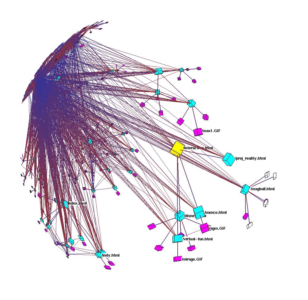
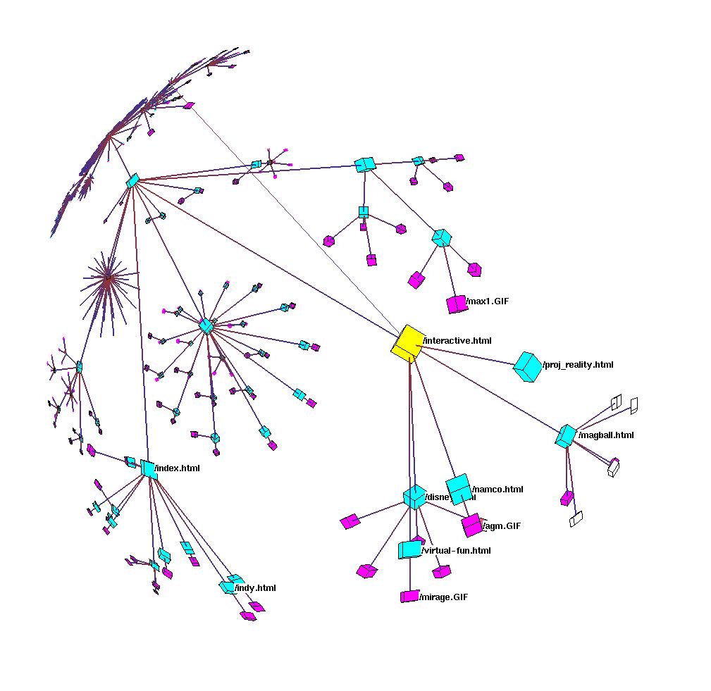
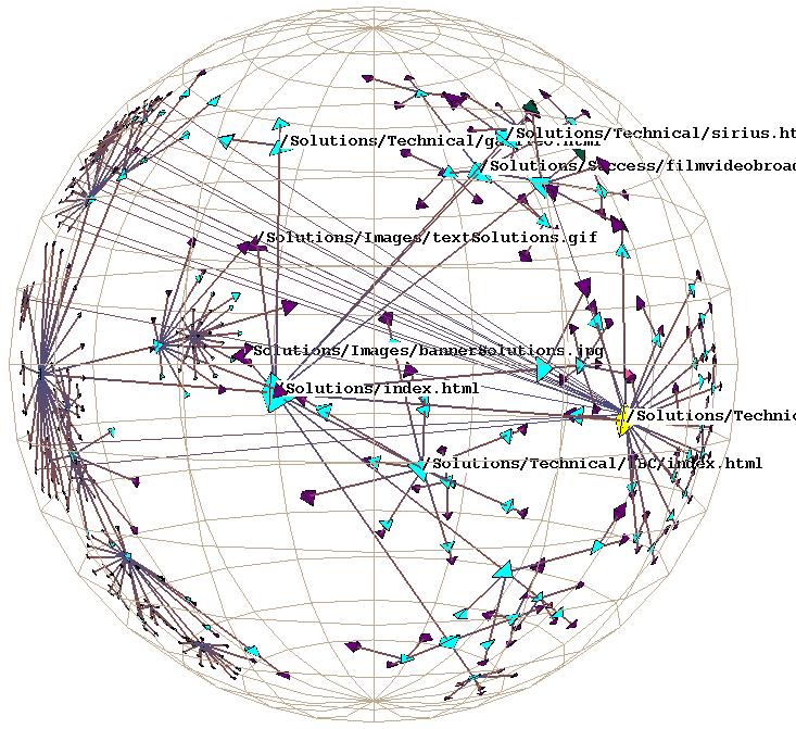
A node can have multiple attributes, and each attribute can be set to a value. These values are the groups. One attribute could be used to control whether a node is drawn, while a different attribute could be used for coloring. For instance, in Figure 3.22 each of the nodes (which represent web documents) has been assigned a value for two distinct attributes. The document type attribute is used for coloring: the value HTML is colored cyan, the image value is colored purple, the VRML value is blue, and so on. Another attribute is location, which is used to filter node drawing. Local nodes are drawn, whereas external nodes are hidden.
The attribute-value mechanism gives the application user explicit control over grouping nodes. In contrast, links fall into one of two more fundamental groups: spanning tree links and non-tree links. These groupings are not explicitly specified by the users, although they can be indirectly controlled by the user's choice of spanning tree algorithms. Spanning tree links are always drawn. The non-tree links are drawn on demand, either for a particular node or for an entire subtree, for a fine-grained control of the display. The directionality of all links can be indicated by gradually interpolating between one color at the parent end and another at the child end. The default coding (changeable through the API) uses a subtle red to blue coding. This color coding is non-intrusive when only the spanning tree is shown, but allows the user to distinguish between incoming links and outgoing links when non-tree link drawing is enabled.
The first implementation of the H3 layout algorithm was deployed before we developed the H3Viewer drawing algorithm. The application was written in C++ and used a highly modified version of Geomview [PLM93] for the drawing engine. The user needed to explicitly expand or contract subtrees, since this gardening was not automatically invoked by navigation. The original PARC cone tree system [RMC91] also used explicit gardening controls.
The next version of the system featured an OpenGL implementation of the H3Viewer guaranteed frame rate drawing algorithm. The adaptive drawing routines incorporated automatic subtree expansion and collapse, obviating the need for manual gardening by the user. We incorporated both the H3Viewer drawing and the H3 layout code into a callable library with a documented API.
The H3 layout and H3Viewer drawing libraries have been integrated into
Site Manager, a commercial product from Silicon Graphics that was
bundled with Irix.![]() Site Manager was designed to aid webmasters and content creators in web site creation and maintenance. The
visualization component was integrated with components for version
control, editing, previewing, and log file analysis.
Site Manager was designed to aid webmasters and content creators in web site creation and maintenance. The
visualization component was integrated with components for version
control, editing, previewing, and log file analysis.
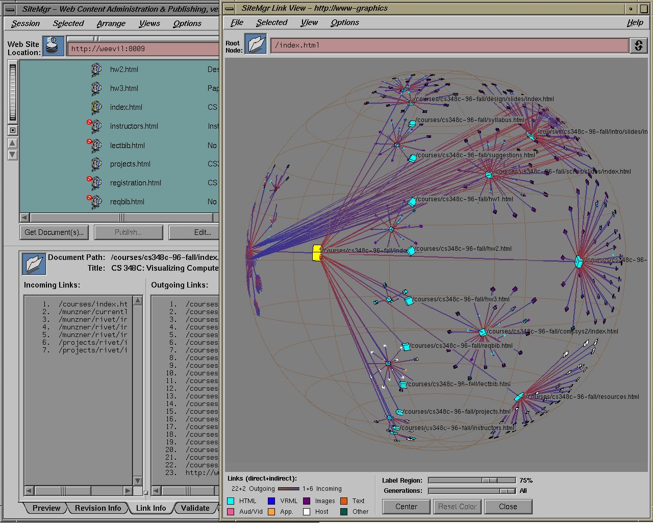
Figure 3.15: Site Manager. The Site Manager product for webmasters from SGI incorporated the H3 and H3Viewer libraries. The 3D hyperbolic view of the hyperlink structure of the web site is tightly linked with a traditional 2D browser view of its directory structure. Figure 3.20 shows the same dataset in a standalone viewer.
Figure 3.16: Linked views. The H3 library allows brushing. The highlighted subtree in the H3 view on the right shows the spatial proximity of a set of documents laid out according to their hyperlink structure, whereas the visible nodes in the directory view on the left that were highlighted because of the link are not all spatially proximate. Also, the HTML preview in the lower left corner was triggered by direct manipulation of the subtree parent node in the H3 view.
Figure 3.17: Traffic log playback. The Site Manager application controls the linked H3Viewer window through the API, so that each hit from the site's traffic log triggers an animated transition and a series of color and linewidth changes. The result looks like the source document fires a laser beam at the destination, which ends up slightly hotter afterward. The nodes are all colored grey at the beginning of the playback, and by the end the most popular documents are a fully saturated red.
In section 3.1.1.1 we discussed the value of linking an interactive graph browser to other views of the data. The Site Manager system mentioned earlier is an example that features a tight integration between the 3D hyperbolic graph browser and several other views of the web site dataset. The screen snapshot in Figure 3.15 shows part of the Stanford Graphics Group web site on display during a Site Manager interactive session. The 3D hyperbolic graph view shows the hyperlink structure of the site, which is linked with the 2D browser view that shows the directory tree structure in traditional outline format. When a node is selected in one view, it is highlighted and moved to the center in both. If several nodes are selected at once, by rubberbanding in the outline view or selecting an entire subtree in the graph view, they are highlighted in both but no motion occurs. The support for brushing allows users to correlate information across views, as shown by the cyan circles in Figure 3.16. The figure also demonstrates how linked views can trigger functionality in other software components through direct manipulation of a graph view, since clicking on the parent node in the subtree resulted in an HTML preview of the associated document in the lower left corner.
The H3Viewer is optimized for browsing, but the tradeoff is that it is quite frustrating to search by navigation for a node when the user knows the name but its spatial location. Applications built for tasks where searching by name is desirable should link the H3Viewer window with a user interface element suitable for handling search, and use the H3Viewer library API to trigger highlighting and animated transitions as appropriate. The Site Manager application has a search window with an input field for typing a query term and a display for the URLs returned by the query. Clicking on a result in that display triggers selection and animated transition in the H3Viewer. The user can then use the navigational capabilities of the H3Viewer to investigate the local area.
Another example of the power of linked views is shown in Figure 3.17. The Site Manager application can analyze a web site's traffic logs. The analysis window on the lower right contains a flat list of the most popular pages. The H3Viewer window on the right is being controlled through the API to show a hit by hit playback of the traffic logs. Instead of being colored by MIME type, the documents are being gradually colored according to their popularity on a color scale with a saturation ramp ranging from grey to red, as shown in the key in the bottom left of the H3 window. At the beginning of the playback, all nodes are initialized to grey. Each hit recorded in the logs triggers a series of color changes: first the source node, then the link between the source and destination nodes, and finally the destination node turns yellow. Then the source returns to its original color, and the destination permanently changes color to a slightly more saturated red. Since the color changes occur in quick succession, the visual effect is a source shooting a laser beam at a destination, making it hotter on each hit. The user can choose to have the destination mode always animate to the center so that the user's activity is always visible instead of being potentially lost in the fringe, or retain navigational control if the goal is to understand the traffic in a local area. The user can also choose to have the affected links stay yellow to leave trails that persistently show hits, even those that were not on the spanning tree. As we discussed in section 3.1.1.1, showing the choice actually made by the user in the context of all available hyperlink possibilities provides a detailed picture of user activity that is hidden in the simple flat list of aggregate popularity.
Linking an H3 window to additional windows or user interface elements can
also make better use of screen real estate than a standalone radial
layout -- a solo H3 window subtends a square instead of a rectangle
with the dimensions of the standard 4:3 monitor aspect
ratio.![]()
Although the layout described in section 3.2 uses
hyperbolic distances, we must eventually project from hyperbolic to
Euclidean coordinates so as to actually draw a picture with
standard low-level graphics libraries.![]() The stage in the algorithm at which this conversion
takes place has a
major effect on the size of the static structure that can be displayed
without encountering precision problems. Distinct hyperbolic
coordinates that are too far from the origin will be projected so
close to the surface of the unit ball that there are not enough bits
to distinguish between their Euclidean coordinates. Such nodes are far
from the root and project to an area much smaller than a single pixel.
The limit comes into play only if we store a static structure in
Euclidean coordinates that is much larger than the part that is
actively being drawn.
The stage in the algorithm at which this conversion
takes place has a
major effect on the size of the static structure that can be displayed
without encountering precision problems. Distinct hyperbolic
coordinates that are too far from the origin will be projected so
close to the surface of the unit ball that there are not enough bits
to distinguish between their Euclidean coordinates. Such nodes are far
from the root and project to an area much smaller than a single pixel.
The limit comes into play only if we store a static structure in
Euclidean coordinates that is much larger than the part that is
actively being drawn.
In our current implementation we do store a static structure: we project immediately after the layout phase, and then change the focus from one part of the structure to another by applying a transformation to the static structure. Any single mapping from hyperbolic to Euclidean space permits drawing only a limited number of nodes before the drawing system succumbs to precision problems.
In the first Geomview implementation, nodes that were too far from the current root of the tree were simply truncated, and could be seen only if by reloading a new input file where the root used to compute the spanning tree was changed. Moving from single to double precision extended the viewable range, but was only a stopgap improvement.
The current version of the H3Viewer drawing algorithm partially addresses the precision problem. The automatic expansion and contraction tied to the navigation allowed users to productively view datasets large enough that the precision horizon was actually reachable. The H3Viewer system will compute a remapping from hyperbolic to Euclidean space as necessary when the cumulative error becomes too great. This remapping is a global operation that depends on the total number of nodes in the scene instead of only the visible nodes. When drawing large graphs, this remapping will cause a temporary interruption in the otherwise smooth frame rate or a jump instead of an animated transition. This remapping is the only exception to our frame rate guarantee.
A more sophisticated implementation could defer the projection until render time and dynamically determine the appropriate Euclidean coordinates for only objects in the neighborhood around the focus that are large enough to see. An incremental mapping algorithm along these lines is possible future work.
The Site Manager application is bundled with Irix 6.2-6.5, and can
also be downloaded for free.![]() It runs only on SGIs.
It runs only on SGIs.
The H3 and H3Viewer library source is available for free noncommercial
use.![]() The
software was written in C++ and OpenGL, so it will run on any machine
that has OpenGL (or Mesa), including Windows and most Unixes. The
library distribution includes an example application of a simple
standalone graph viewer.
The
software was written in C++ and OpenGL, so it will run on any machine
that has OpenGL (or Mesa), including Windows and most Unixes. The
library distribution includes an example application of a simple
standalone graph viewer.
Static pictures such as figures in this paper could be misinterpreted as showing 2D objects on the surface of a hemisphere instead of as 3D objects inside the volume of a ball. In the interactive system the dimensionality is obvious when the objects rotate inside the ball.
The main way for users to navigate is by simply clicking on a node or edge. When the user clicks on a node, it is selected and undergoes an animated transition to the center of the sphere. The frame rate during an animated transition is guaranteed to be constant, just like the frame rate during explicit user navigation. The transformation includes both a translation to move the node from its old position to the origin, and a rotational component to position the node so that its ancestors are all on the left side and its descendants are all on the right. This configuration provides a canonical local orientation. We add a slight tilt so that the ancestor-descendant axis is not perfectly horizontally aligned with the principal axis of the window, so that the text labels are less likely to occlude each other.
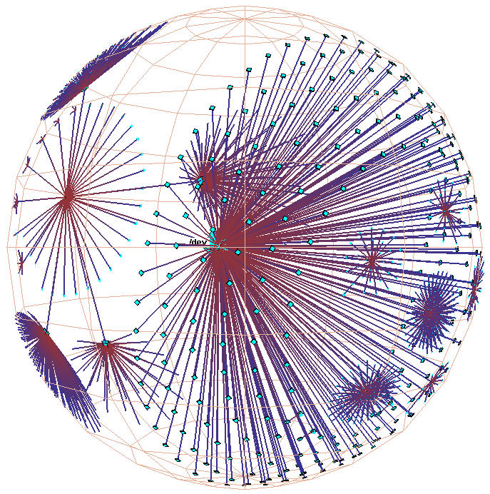
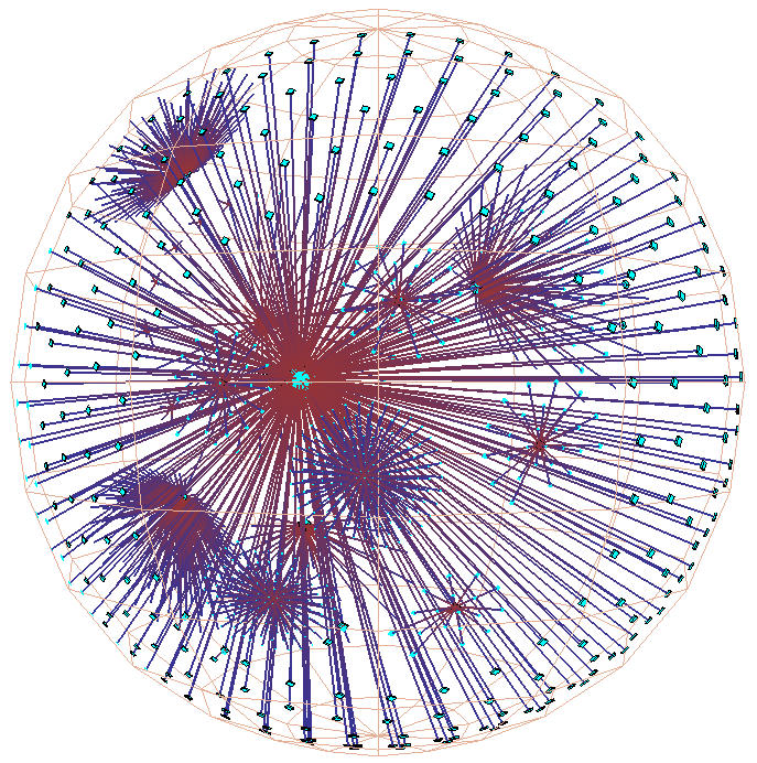
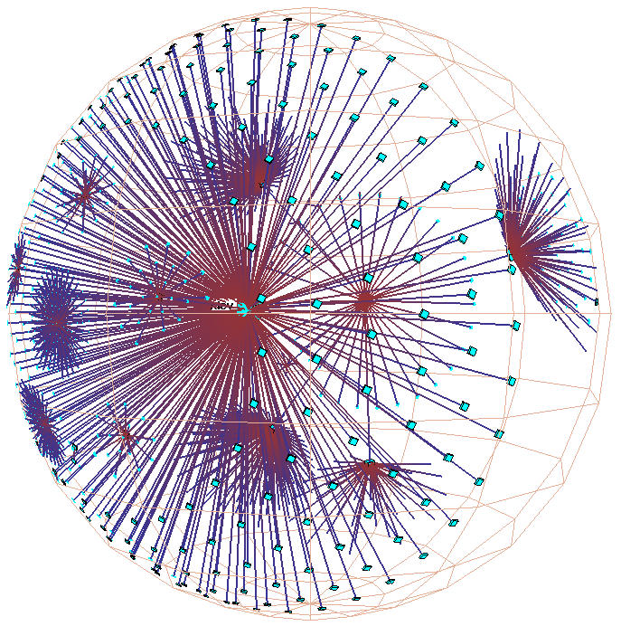
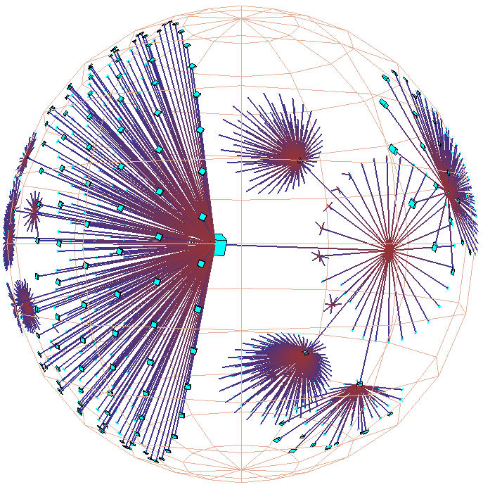
Figure 3.18: Hyperbolic motion over a 30,000 element Unix file system. Many nodes and edges project to subpixel areas and are not visible. Top row: Translation of a node to the center. Bottom row: Rotation around the center node. The rotation clarifies that objects lie inside a ball, not on the surface of a hemisphere. The file system has a strikingly large branching factor when compared with the web sites in Figure 3.20 or the call graphs in Figure 3.21. The directory that approaches the center, /usr/lib, contains a large number of files and subdirectories.
If the user clicks on an edge, that point is translated to the center of the sphere but no rotation or selection occurs. The user can also rotate the structure around the origin of the ball, which spins everything around the current focus node. Finally, power users can have explicit control over hyperbolic translation through mouse drags. Figure 3.18 shows a multi-image sequence of hyperbolic translation.
Non-tree links, which are in the original graph but not in the computed spanning tree, do not affect the layout. These non-tree links are drawn by simply connecting the two nodes that have been laid out in the tree structure. We do not explicitly check for edge crossings because our tree layout makes such a crossing in 3D space highly unlikely.
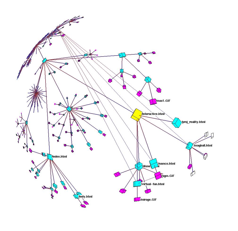


Figure 3.19: Non-tree links. Top left: Drawing all the non-tree links for dense quasi-hierarchical graphs results in an incomprehensible mess. Top middle: The spanning tree alone is quite clear. Top right: The node highlighted in yellow near the center has a single incoming non-tree link. Bottom left: The entire subtree beneath that node has more incoming non-tree links. Bottom middle: The highlighted yellow node has many outgoing non-tree links. Bottom right: Drawing the outgoing non-tree links for the entire subtree beneath the highlighted yellow node shows the highly interconnected nature of the web site without overwhelming the viewer with a mass of links.
Although the spanning tree links are always drawn, the non-tree links are drawn only on demand. The top left image of Figure 3.19 shows why: a typical web site with all the non-tree links drawn results in an incomprehensible mess. The ability to interactively select which non-tree links are drawn is critical for making the H3 layout useful with dense quasi-hierarchical graphs. The user can draw incoming or outgoing non-tree links on demand for any node or subtrees. The rest of Figure 3.19 compares the visual effect of these controls. In the Site Manager application, we explicitly distinguish between entering and leaving links categories in the user interface, but other application programmers might choose to hide this API distinction if such fine-grained control is unnecessary for their target task.
Our implementation can handle graphs two orders of magnitude larger than most previous systems by manipulating a backbone spanning tree instead of the full graph. Carrying out both layout and drawing in 3D hyperbolic space lets us see a large amount of context around a focus point. Our layout is tuned for a good balance between information density and clutter, and our adaptive drawing algorithm provides a fluid interactive experience for the user by maintaining a guaranteed frame rate.
We begin by discussing the visual appearance of several datasets under the H3 layout, followed by an analysis of the layout algorithm speed and scalability that is both quantitative and qualitative. We next discuss a user study conducted at Microsoft Research that found a statistically significant improvement in task time when a novel web browser that included the H3Viewer was compared to more traditional browsers. We then present several additional task domains where H3Viewer was used, and conclude by summarizing the outcomes of the project.
Figure 3.20: Part of the Stanford graphics group web site drawn as a graph in 3D hyperbolic space. The entire site has over 14,000 nodes and 29,000 edges. About 4000 nodes in a 7-hop diameter neighborhood of the papers archive are visible in this snapshot. One dozen of the nodes are labelled, a few hundred more have visible color coding or are individually distinguishable, and the rest of the nodes on the fringe provide aggregate information about their presence or absence. In addition to the main spanning tree, we draw the nontree outgoing links from an index of every paper by title. The tree is oriented so that ancestors of a node appear on the left and its descendants grow to the right.
The H3 layout technique can easily handle tens of thousands of nodes and has been tested on graphs of over 100,000 nodes. It is highly effective at presenting a large neighborhood around a focus node of a huge graph in a small amount of screen space. For instance, in Figure 3.20 the user can see enough of the distant subtrees to identify dense and sparse ones. The destinations of nontree links are distorted, but the rough sense of their destination helps the user construct and maintain a mental model of the larger graph structure. Figure 3.18 shows how the details become clear in a smooth transition when an area of the structure moves towards the center. The context shows up on several levels: the local parent-child relationships of the spanning tree, the nontree links between disparate nodes in the graph, and the rough structure far away from the current focus of interest.
Figure 3.21: Call graph. We show the static function call graph structure for a mixed C and FORTRAN scientific computing benchmark. On the left the node coloring indicates whether a particular global variable was untouched (cyan), referenced (blue), or modified (pink). On the right we use the same color scheme with a different variable. Such displays can help software engineers see which parts of a large or unfamiliar program might be modularizable.
Figure 3.21 shows our layout techniques at work on one of the function call graphs described in section 3.1.1.3 instead of the web sites shown in many of the other figures.
Figure 3.22: Link structure of a web site laid out in 3D hyperbolic space. We show the link structure of a web site laid out in 3D hyperbolic space. The nodes represent documents, which are colored according to MIME type: HTML is cyan, images are purple, and so on. We draw the outgoing non-tree links for the selected node, highlighted in yellow. Top: The destination of the outgoing links is quite distorted, but we do see that most of the links end at a particular cluster. Bottom left: We drag that cluster towards the focus to see more detail. Bottom right: The cluster is close enough to the center to see individual destination nodes.
Figure 3.22 shows a medium sized web site that contains 5000 total nodes. The top image shows a selected node with outgoing nontree links drawn. Although distant subtrees are quite distorted, we can see enough context that the destinations of the non-tree links can be roughly distinguished. In the other two images we bring the cluster of nodes that contains the destination of most of the nontree links closer to the focus. Note that we can still see the originating node, although it is quite far away in the tree structure.
The H3 layout algorithm is linear in the number of spanning tree
edges. Adding an edge to the spanning tree is a constant amount of
work, and every edge addition requires one comparison, so the
spanning tree creation is order |E| (the number of edges in the
graph). In the current implementation the required input file format
is a depth-first traversal of a graph with an explicitly declared
root.![]() The
node layout algorithm depends on only the spanning tree structure, not
the underlying graph structure. The top-down placement pass is order
|V|, the number of vertices in the graph, since placing the child
hemispheres on the parent requires only one computation per node. The
bottom-up estimation pass where we sum over the child nodes is also
order |V|. On an SGI Onyx2 a large graph with 110,000 edges was laid
out in 12 seconds, a medium sized graph of 31,000 edges was laid out
in 4 seconds, and a small graph of 4000 edges took a fraction of a
second.
The
node layout algorithm depends on only the spanning tree structure, not
the underlying graph structure. The top-down placement pass is order
|V|, the number of vertices in the graph, since placing the child
hemispheres on the parent requires only one computation per node. The
bottom-up estimation pass where we sum over the child nodes is also
order |V|. On an SGI Onyx2 a large graph with 110,000 edges was laid
out in 12 seconds, a medium sized graph of 31,000 edges was laid out
in 4 seconds, and a small graph of 4000 edges took a fraction of a
second.
The drawing time is constant - the H3Viewer drawing algorithm always maintains the target guaranteed frame rate. A slow graphics system will simply show less of the context surrounding the node of interest during interactive manipulation. Figures 3.13 and 3.14 show two views of the same scene - one corresponding to what the user would see during interaction, and one after the fringe has been filled in when the user was idle. On startup, the initial loading phase includes both file I/O and data structure building. For the graphs mentioned in the previous paragraph, this time was approximately 2 minutes, 20 seconds, and 2 seconds, respectively.
The layout and drawing algorithms presented here work well up to the
limits of main memory, but not beyond: if the entire graph does not
fit into main memory, the system is unusable. The graph with 110,000
edges could be manipulated interactively on an SGI with 1 GB of main
memory but could not be loaded on a smaller 128 MB
machine.![]() Thus, the obvious computational limit on H3 scalability is
main memory. Although the drawing algorithm uses only information
about a local area, the layout algorithm is global. The precision
problem discussed in section
3.5.2 is also a limit on the current implementation,
albeit not on the algorithm itself.
Thus, the obvious computational limit on H3 scalability is
main memory. Although the drawing algorithm uses only information
about a local area, the layout algorithm is global. The precision
problem discussed in section
3.5.2 is also a limit on the current implementation,
albeit not on the algorithm itself.
However, we have also found cognitive factors that limit its scalability, and these factors cannot be solved by simply adding more memory to a machine or tightening the memory footprint of the software. Depending on the characteristics of the dataset, the local visible neighborhood around a focus point in H3 is between five and twelve hops. Although this is a much wider local view than previous systems, it is nevertheless not a global overview. The distinction is blurred in datasets of moderate size, but becomes clearer as the size of the dataset increases. People can easily become disoriented when the H3Viewer displays huge datasets of over 100,000 nodes. The important factor in retaining orientation is the ability to relate the currently visible neighborhood to the entirety of the graph, which is related to the diameter and branching factor of the graph as opposed to the sheer number of nodes. We conjecture that disorientation sets in when the diameter is over an order of magnitude larger than the visible neighborhood.
The combination of a carefully tuned layout and interaction allowed us
to push the limits of large graph browsing far beyond their previous
place of a few thousand nodes. We conjecture that the reach of H3
could be extended by adding landmarks to the scene, perhaps so that
the direction of a path back the root node was always obvious. Another
possibility would be to link an H3 window with a true global overview
window, perhaps based on the skeletonization work of Herman and colleagues
[HMM 99]. One way to extend the existing H3 implementation to much
larger datasets would be by using multiple linked H3 windows to
explore the dataset at more than one discrete levels of detail:
clicking on a node in a higher-level window would cause its subgraph
to be displayed in another window. This scheme could probably scale to
a few levels of recursion before disorientation set in.
99]. One way to extend the existing H3 implementation to much
larger datasets would be by using multiple linked H3 windows to
explore the dataset at more than one discrete levels of detail:
clicking on a node in a higher-level window would cause its subgraph
to be displayed in another window. This scheme could probably scale to
a few levels of recursion before disorientation set in.
Figure 3.23: XML3D interface. The XML3D browser, which combined an H3Viewer window with several auxiliary lists, was compared with two traditional web browsers during a user study. XML3D was reliably faster for some tasks and had equivalent performance for others. Image courtesy of Mary Czerwinski, Microsoft Research.
Kirsten Risden and Mary Czerwinski of Microsoft Research ran an empirical study [RCMC00] comparing three web browsers, one of which incorporated the H3Viewer libraries. The user study demonstrated the strengths and weaknesses of three browsers. Two were conventional 2D browsers: a standard collapse-expand tree browser of the form found in many Windows applications, and a web-based hierarchical categorization from the snap.com portal (which is similar to Yahoo!). The third browser was XML3D, a novel browser that integrates an H3-based interactive 3D hyperbolic graph view with a more traditional 2D list view of the data. The focus of the study was browser designs that could help organize, make sense of, and manage large collections of documents available on the Web. We were were particularly interested in collections that are not strictly hierarchical in structure. Our target user population deals with non-hierarchical datasets, where categories may have one or multiple parents, on a daily basis in the course of Web site content generation and maintenance.
XML3D is capable of graphically representing the information contained within schema-like, XML text files. The interface consists of two types of linked components: an instance of the H3Viewer and several 2D lists -- of parents, children, and siblings -- which dynamically update based on the selected graph node. XML3D also includes a history list and search capability. In Section 3.5.1, we asserted that the H3Viewer is most powerful when effectively linked with other interface components. XML3D was built to explicitly test this assertion in a particular task domain, that of Web content developers and maintainers, our target audience. Figure 3.23 shows an example of the XML3D application.
We had access to the 12,000 node categorization hierarchy which was available from the snap.com portal, and ported its contents into XML3D and a 2D collapsible tree browser. We used the live Snap.com hierarchy as the second 2D alternative during the study. Tasks with different levels of complexity were created by varying: (1) whether the subject was asked to find an existing category or add a new category to the directory scheme; and (2) whether the target category and requested response involved a single parent path or multiple parent paths. The tasks varied in kind as well as complexity across levels.
Figure 3.24: XML3D vs. 2D interface study results. In the user study we empirically compared the usability of XML3D to two established 2D interfaces: a collapsible tree browser such as appears in many Windows applications, and the click-through user interface of a Web portal. The two pairs of bars on the left side of the figure show the performance differences for the task of adding documents to an existing category, and the difference between the XML3D interface and the 2D interfaces is statistically significant. The two pairs of bars on the right side shows the performance differences for the task of creating an entirely new category in which to place a document, and these differences are not statistically significant. (Image courtesy of Mary Czerwinski, Microsoft Research.)
Figure 3.24 shows the task time results. We did not observe any reliable differences in task times between the two 2D browsers, so they are combined into a single category. The significant variable was the task type: adding content to existing categories vs. creating new categories. The results showed clear differences between XML3D and the 2D interfaces. With XML3D, participants performed search tasks within existing categories reliably faster with no decline in the quality of their responses. In the new category search task, there was no reliable overall difference. Interestingly, a breakdown of user activity logs indicates that in this no-improvement new category task case, users made little use of the XML3D interface component, spending most of their time interacting with the 2D list components. In the performance-improvement existing category task case, their time was roughly equally split between the interface components.
We can explain Figure 3.24 more formally: analysis
of variance on mean task completion times revealed main effects of
user interface condition (XML3D vs. 2D),  ,
,  ,
and category (new vs. existing),
,
and category (new vs. existing),  ,
,  .
Participants completed tasks faster using XML3D than using the more
conventional interfaces. In addition, participants were faster to
complete tasks involving an existing as opposed to a new category. The
main effect of category was qualified by a significant interaction
with the parent variable,
.
Participants completed tasks faster using XML3D than using the more
conventional interfaces. In addition, participants were faster to
complete tasks involving an existing as opposed to a new category. The
main effect of category was qualified by a significant interaction
with the parent variable,  ,
,  . Follow-up
analyses showed that the difference between existing and new category
tasks was larger when a single parent was involved,
. Follow-up
analyses showed that the difference between existing and new category
tasks was larger when a single parent was involved,  ,
,  , than when multiple parents were involved,
  ,
,  . Neither the main effect of parent nor any of the other
interactions were significant.
. Neither the main effect of parent nor any of the other
interactions were significant.
There were no reliable differences in overall user satisfaction or consistency across the three user interface designs. In other words, the benefit in performance in the XML3D case was not offset by a lack of agreement across users as to where web content should be placed. It was informally observed that integrating the ability to view the overall structure of the information space with the ability to easily assess local and global relationships was key to successful search performance. XML3D was the only tool of the three that efficiently showed the overall structure within one visualization.
Future studies should explore optimal ways of integrating the use of novel 3D graph layouts and 2D lists for effective information retrieval, so that other kinds of tasks might benefit from the new designs. Nevertheless, we have seen that giving users the option to use a novel visualization in addition to a traditional 2D list view appears to be a powerful design solution, at least until alternative user interfaces become more pervasive.
The H3 system was the most successful of the three projects by several of the evaluation metrics discussed in section 1.3.2.1: user studies, tangible algorithmic improvements compared to previous systems, and size of user community. The preceding section contains the details of the performance advantage for an H3-based system found in the user study. We have presented a layout algorithm that scales linearly to datasets 100 times larger than almost all previous systems and a drawing algorithm that guarantees a constant frame rate. The potential user community is large because H3 was incorporated into a commercial product.
One of our motivations for integrating the research software with a product was the hope of getting feedback from a large user community. Our previous experience with large software projects was as one of the core developers of Geomview [PLM93], a public domain 3D interactive graphics package that explicitly solicited user response in its documentation, which generated considerable feedback. Site Manager instead followed the pattern of a commercial product release, which does not establish channels of communication between the developers and the users. Thus, we have no data on the size and satisfaction level of the commercial users.
However, we have had communication from noncommercial H3Viewer users.
SGI funded the development of the H3 and H3Viewer code base, but
agreed to allow us to release the libraries for free noncommercial
use. The software has been publicly downloadable![]() since 1999, and was also
privately released to a limited number of interested researchers
between 1997 and 1999. The following section covers these additional
task domains.
since 1999, and was also
privately released to a limited number of interested researchers
between 1997 and 1999. The following section covers these additional
task domains.
The H3 system has been used for many kinds of data in addition to web hyperlink structure. Our collaboration with the SUIF compiler group to incorporate an H3 view of function call graphs into their development environment had a promising start, but was cut short when the key contact person left their group. Several researchers have converted their datasets into the H3Viewer format to use the simple standalone viewer to browse through their data. A representative example is Dave Vieglais of the Natural History Museum and Biodiversity Research Center at the University of Kansas, who wanted to see species taxonomy data. Such a project involves a minimal investment of researcher time, on the order of hours or days.
A more significant investment of time, on the order of weeks or more, was required from the researcher who incorporated the H3 libraries into his own software system. Daniel W. McRobb of the Cooperative Association for Internet Data Analysis (CAIDA) did so for two problem domains in networking: Internet tomography and BGP peering relationships.
Skitter![]() is a
project from CAIDA to develop and deploy active measurement tools for
the dynamic discovery and depiction of global Internet topology and
for measuring performance across specific paths. The project goals are
acquiring infrastructure-wide connectivity information, collecting
round trip time and path data for up to 60,000 destinations, and
analyzing the visibility and frequency of routing changes. The Skitter
team tried several methods of visualizing their large datasets,
including Cheswick and Burch's software
is a
project from CAIDA to develop and deploy active measurement tools for
the dynamic discovery and depiction of global Internet topology and
for measuring performance across specific paths. The project goals are
acquiring infrastructure-wide connectivity information, collecting
round trip time and path data for up to 60,000 destinations, and
analyzing the visibility and frequency of routing changes. The Skitter
team tried several methods of visualizing their large datasets,
including Cheswick and Burch's software![]() , and have settled on the
H3Viewer as the more effective approach for their needs as of yet.
They built a custom software tool for browsing this dataset that
incorporates the H3Viewer libraries.
, and have settled on the
H3Viewer as the more effective approach for their needs as of yet.
They built a custom software tool for browsing this dataset that
incorporates the H3Viewer libraries.
Figure 3.25: Autonomous System paths analysis. Images and (edited) caption courtesy of Daniel W. McRobb, CAIDA. The displayed spanning tree represents connectivity seen from pinot.caida.org on March 3, 1999. Top left: ALPHA-NAP is the root where we captured the AS path data. Top right: Here we clicked on the node at the center of the cluster in the bottom of our first view. Hypviewer brings the node to the front and center, and we see that this AS is the vBNS. Bottom left: Again following the large clusters, we clicked on the node at the center of the large cluster behind the vBNS, and found Cable and Wireless (CWUSA). Bottom right: Here we clicked on one of the small clusters off of CWUSA and found Verio. Since we're in a fairly small neighborhood, we see many labels.
McRobb has also used H3 to explore the peering relationships between
the Autonomous Systems (ASes) that constitute the backbone of the
Internet. The routing relationships between Autonomous Systems are
notoriously complex because the policies that can be set via the
Border Gateway Protocol. Visualizing these graphs is particularly
challenging for many systems because of the large branching factor for
many of the nodes. The H3 layout is able to handle these large
datasets, and the guaranteed frame rate drawing algorithm is critical
for exploring them in real time. Figure 3.25 shows McRobb's
analysis of Autonomous System data gathered using the mrtd
tool.![]() (Figure 3.13
on page
(Figure 3.13
on page ![]() also shows Autonomous System data, from a
different source.)
also shows Autonomous System data, from a
different source.)