A Practical Introduction to
Light Field Microscopy

Zhengyun Zhang

Contents

• Setup
  • What are the components in a light field microscopy system?
  • What design choices are there in a light field microscopy system?
  • What's one way to build a light field microscope?
  • How do I calibrate the system?
    • How do I make sure the camera is imaging the back focal plane of the microlens array?
    • How do I align the microlens array to the intermediate image plane?
  
  
• Usage
  • How do I install the software?
  • How do I stream from a camera in LFDisplay?
  • How do I calibrate LFDisplay for light field imaging?
  • How do I interactively explore a specimen?
  • How do I save and load image data in LFDisplay?

Setup

Light field microscopy is a useful tool that allows microscopists to collect three-dimensional information about a scene in a single snapshot. Let us first look at what comprises a light field microscopy system and what design choices are involved. Next, we'll walk through the required materials and step-by-step instructions on a specific light field microscope system. Lastly, we'll look at how to calibrate that particular design, along with notes on how to calibrate light field microscope systems in general.

What are the components in a light field microscopy system?

Figure 1.1: A light field microscope is created by inserting a microlens array (D) of focal length $f_3$ at the intermediate image plane of an optical microscope consisting of an objective (B) with focal length $f_1$ and tube lens (T) with focal length $f_2$. The sensor (E) is now placed at the back focal plane of the microlens array. The different ray bundle diagrams correspond to paraxial rays from points in the specimen (a), axial rays from specimen (b), all rays from a single point in the specimen (c), and several discrete ray angles which reach a single microlens (d).

(a)

(b)

(c)

(d)

A light field microscopy system consists of the following:

• an optical microscope,
• a microlens array,
• (optional) relay lenses,
• a digital camera,
• and postprocessing software.

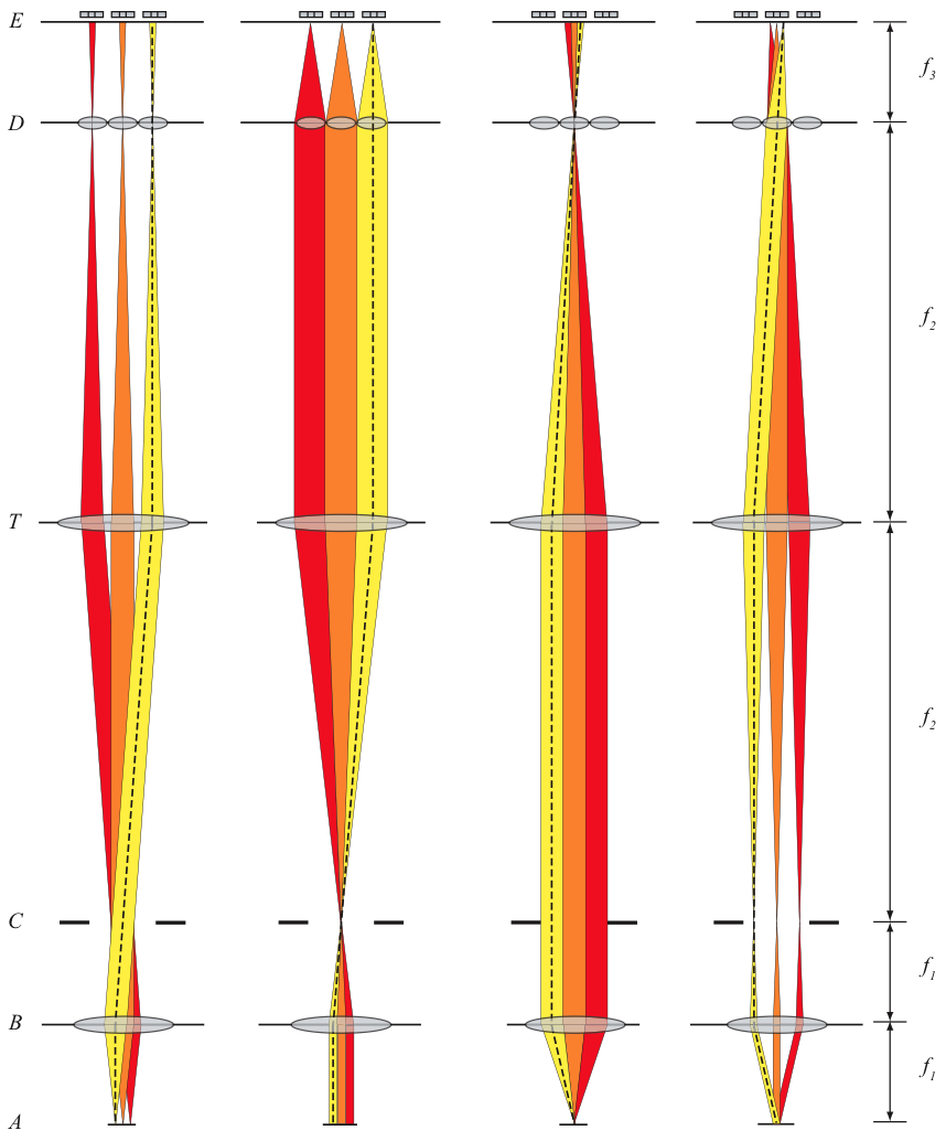
A standard optical microscope imaging system can be converted into a light field microscopy system with the addition of a microlens array and postprocessing software. An optical diagram is shown in Figure 1.1 denoting the various lenses, stops and sensors in the system. The microlens array is inserted at the original intermediate image plane, where the camera would originally focus for standard microscopy. The camera itself is moved back so that it focuses on the plane one focal length behind the microlens array (the back focal plane). The camera produces raw light field images consisting of a lattice of small circles, which are then processed by postprocessing software to either allow interactive exploration of a specimen or to create focal stacks for further analysis.

What design choices are there in a light field microscopy system?

The main aspect of light field microscopy system design is that of the microlens array, although other things such as choosing a camera, designing a housing for microlens arrays and choosing an objective are also important.

The first thing you should ask yourself when designing a light field microscopy system is: what's the smallest feature size I need to be able to resolve in the final output? For example, you might want to be able resolve neurons that are five microns across in size. Remember that you cannot push this feature size too small, or you will lose the ability to refocus due to the diffraction limit, as explained in the previous section.

Next, you should determine what objective you would like to use. The main choice here is really for the field of view, as opposed to smallest resolvable spot. You want to determine how much of the specimen you need to be able to image at once, and hence should probably choose an objective with the highest NA that is both appropriate for your specimen and will be able to image a field large enough.

There's often not too much choice involved in obtaining a camera, but if you do have a choice, you should opt for a camera that has as many pixels on the sensor as possible, assuming it fulfills your sensitivity requirements (and framerate requirements for streaming applications). This is because the actual output pixel count in a rendered focused image from a light field is the sensor pixel count divided by the number of pixels that fit inside a single microlens.

As a caveat, the camera and objective choices do affect one another. For example, if the camera sensor doesn't image the entire intermediate image plane, then you might want a lower magnification objective in order to fulfill the field of view requirement. Also, ideally we want the sensor pixel size to be roughly half the size of the diffraction spot size of the objective we chose; if the pixel size is too small, we don't get too much extra information from the light, and if the pixel size is too large, we waste information from the captured light, as we can't resolve the finer angular content in the light field image.

Now that we have chosen an objective, a camera and a feature size, we are ready to look at microlens designs. There are two main parameters involved in the design - the pitch and focal length. As for the shape of the microlenses, we should use microlens arrays composed of abutting square aperture lenses in a lattice.

The microlens pitch should be roughly equal to or smaller than our feature size multiplied by the magnification of the objective. For example, if we want to image five-micron neurons using a 40X objective, we should have a microlens pitch equal to $5\times40=200$ micron at the largest; 100 micron pitch microlenses would be preferable. If you are flexible with feature sizes, then go for a slightly larger microlens pitch to achieve better angular resolution (allows more distinct focal planes from a refocusing operation).

Given a microlens pitch and objective, we can calculate what would be an ideal focal length for the microlenses. Recall that for each microlens in the array, we get an image of the aperture of the objective (back focal plane image), which is usually a circle. Shorter focal lengths yield smaller circles, and if the focal length is too short, you waste pixels on the sensor. Longer focal lengths yield larger circles, but if the focal length is too long, your circles overlap in the light field and the overlapping parts cannot be used in light field rendering. Ideally, we want these circles to almost touch, but still have somewhat of a gap between them (to be resilient to diffraction effects).

Now let's look at how to calculate the focal length to have the circles exactly touching. The sine of the maximum half angle of rays passing through the intermediate image plane is equal to the NA of the objective divided by the magnification. For example, a 40X/1.3NA oil objective will create rays that at most hit the intermediate image plane at a $\theta_{max} = \sin^{-1}(1.3/40) = 1.86$ degree angle. Let us suppose we went with 100 micron microlenses. In order to have the circles abut, we want a ray from the center of the microlens stray 50 microns from the optical axis at a distance from the microlens equal to the focal length. Thus, we can solve for the focal length to be: $f = 50 / \tan(\theta_{max}) = 1540$ microns. This is the maximum focal length we would want to use with this objective and microlens array pitch. Perhaps a $1500$ or $1400$ micron focal length would be a safer bet.

To summarize, in this example, we would want to use a 40X/1.3NA oil objective with a 100 micron pitch microlens array with at most 1540 micron focal length in a light field microscopy system to image 5 micron neurons. However, keep in mind that often constraints will prevent the creation an ideal setup, but as long as the design specifications are in the right ballpark and erring on the right side, then you should be okay. For example, it's okay to have the focal length be shorter than the ideal.

What's one way to build a light field microscope?

One of the first prototypes of a light field microscopy system was constructed from the following:

• a Nikon Eclipse 80i upright microscope with universal epi-illuminator,
• a custom-fabricated microlens array holder,
• a microlens array,
• two Nikon 50mm f/1.4 lenses coupled nose-to-nose,
• a QImaging Retiga 4000R cooled CCD camera with F-mount,
• and a Dell XPS 700 workstation

Figure 1.2: Three parts of a microlens array holder. The yellow part slides with respect to the green part and can be attached to an F-mount lens on one end. The green part holds the microlens array. The blue part slides with respect to the green part and can be attached to the microscope on one end. This particular design was for a Zeiss microscope, but the yellow and green parts are designed to be usable with other microscopes if a new blue part is machined.

Figure 1.3: Design plans for a Nikon-compatible holder. The blue part was what was eventually used in conjunction with the yellow and green parts in Figure 1.2.

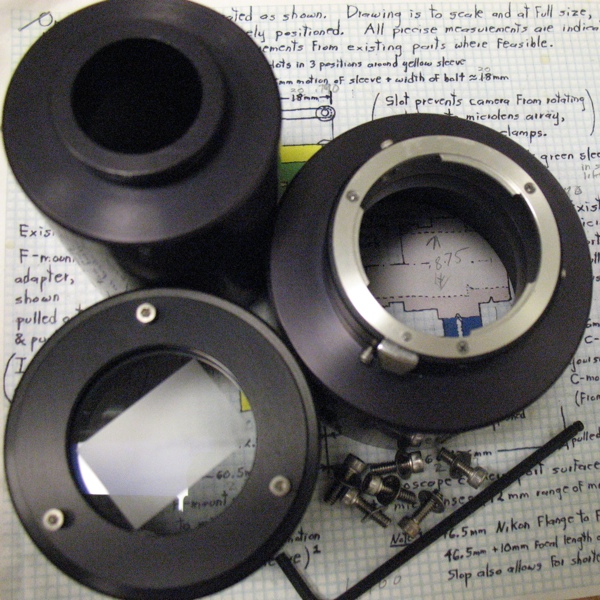
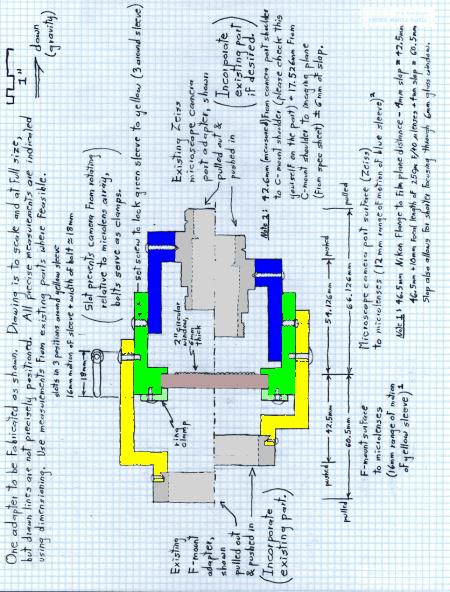
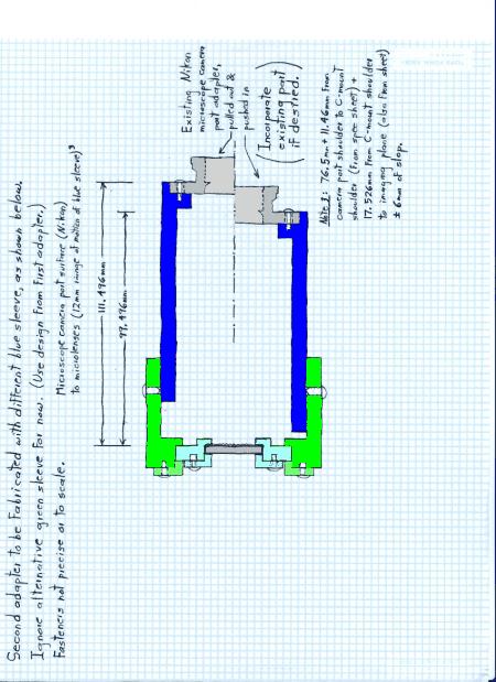
In order to insert the microlens array at the proper height, a microlens array holder was custom machined. The holder for the Nikon microscope consists of the yellow and green sections of the design in Figure 1.2 and the blue section of the design in Figure 1.3. The three pieces of the microlens array holder are:

1. a tube to attach to an F-mount (yellow),
2. a tube that holds the microlens array (green),
3. and a tube to attach to the microscope (blue).

Adjacent tube pieces slide with respect to one another and their positions are locked using three screws. This allows calibration of microlens-to-camera distance and microlens-to-tube-lens distance. The finished, anodized holder pieces can be seen in Figure 1.4.

Figure 1.4: The finished, assembled microlens array holder is shown in (a). The three pieces are shown separately in (b), with a microlens mounted.

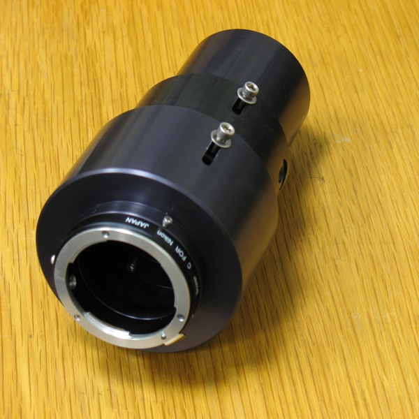
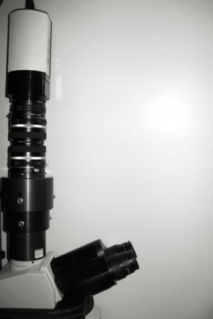
Since the Retiga 4000R's sensor plane is inside a sealed chamber, relay optics are required for the Retiga to be able to focus on the back focal plane of the microlens array. Therefore, two Nikon 50mm f/1.4 prime lenses were connected nose-to-nose using a specialized 52mm filter ring that attached to lenses on both ends. The F-mount on one end attaches to the Retiga and the F-mount on the other end attaches to the microlens array holder. The finished construction can be seen in Figure 1.5

Figure 1.5: The finished light field microscope built on top of the Eclipse 80i. The camera (Retiga 4000R) is connected to the back end of a Nikon 50mm f/1.4 lens. This lens's front is connected to the front of another Nikon 50mm f/1.4 lens using a nose-to-nose filter ring adapter. The back side of the second Nikon 50mm f/1.4 lens is connected to the microlens array holder. Finally, the microlens array holder is attached to the top of the camera port of the universal epi-illuminator.

A Dell XPS 700 workstation was used for this setup. It had a 2.67GHz Core 2 Duo processor from Intel, 2GB of RAM and a Geforce 7900 GTX graphics card from nVidia. The real-time light field imaging application, LFDisplay, and other Python modules for computing focal stacks were developed and installed on this computer. The Geforce 7900 GTX offered decent enough performance, although it was replaced by a Geforce GTX 260 Core216 later after hardware failure.

How do I calibrate the system?

Calibration of the light field microscopy essentially involves two parts:

1. making sure that the camera is imaging the back focal plane of the microlens array, and
2. making sure that the microlens array is conjugate with the intermediate image plane.

We will now outline a sample procedure for calibration, assuming that:

1. the microscope can be used with trans-illumination and has an aperture stop for the condenser, and
2. the microscope allows the user to toggle between a view through the light field microscope (camera mounted on microlens array mounted on camera port) and a non-light field view (eyepiece), and
3. the user can view both views in real time, and
4. optionally, the user can insert a narrow-band red color filter into the imaging system.

The light field microscope system in the previous section fulfills these requirements. However, not all light field microscope systems can be easily calibrated this way, so we encourage you to devise your own calibration schemes using this guide as a reference, as long as they calibrate the two distances specified above. Some possibilities include using epi-reflectance as opposed to transmitted light, attaching a long black tube with a pinhole at the end in lieu of a microscope, or using lenslet circle size/overlap as a metric for correct microlens-to-camera distance.

How do I make sure the camera is imaging the back focal plane of the microlens array?

Figure 1.6: A section of the light field image will look like a normal image with grid overlay (a) if the camera is focused on the intermediate image plane. If the camera is correctly focused on the back focal plane of the microlens array, the image should resemble (b). A red color filter has been used with a monochrome camera for both images, so diffraction ridges in (b) are more apparent than in the case of white light illumination.

(a)	(b)

If the camera does not correctly image the back focal plane of the microlens array, the resulting captured light field image will be blurry if misfocus is by a small amount (resulting in loss of angular resolution) or downright unusable if misfocus is by a large amount. The following is one possible way to make sure the distance between the microlens array and the camera is correct.

1. Place a flat, high contrast specimen onto the stage in Kohler transmitted illumination with the condenser aperture stopped down.

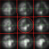
   Since the image behind each microlens is an image of the angular spread of light, the best way to check for focus is to have each microlens try to image a very narrow set of rays. This is accomplished by stopping down the condenser aperture so that the light rays hitting the specimen is roughly parallel to the optical axis. Ideally, we should see a lattice of very small almost point-like plus signs, as shown in image (b) of Figure 1.6. This is the diffraction pattern induced by the microlens array. However, if this is not the case, let us continue with the calibration procedure

2. Optional: Insert a (red) color filter into the system.

   If possible, insert a color filter into the imaging system such that all images are roughly monochromatic. This will help with spotting diffraction patterns later. A red filter is the best, as it produces the largest diffraction patterns. The color filter can either be inserted into the trans-illumination or can be an excitation filter in a filter cube.

3. Adjust the camera-to-microlens distance until you can see a normal image of the specimen with a (light or dark) grid superimposed, as shown in image (a) of Figure 1.6.

   What we have done is to move the camera conjugate plane to the microlens array plane (and not its back focal plane). The microlens edges will cause this grid pattern to appear. This step is not entirely necessary, but it does make it easier to locate the point of best focus, by starting the camera at a known distance from the microlens array.

4. Slowly increase the camera-to-microlens distance until the contents of each ``grid cell'' in the previous step form the smallest point-like pattern possible.

   The total amount of movement required here should be approximately equal to the focal length of the microlens array. Once the image you see from the camera resembles image (b) of Figure 1.6, you are now at the proper position. Note that if your camera pixels are rather large, or if you have not inserted an optional color filter into the microscope, you may not see clear diffraction ridges or the plus sign shape at all. In that case, aim for the smallest sized spot, or adjust until the center pixel of each spot has the highest brightness.

5. Optional: Rotate the camera with respect to the microlens until the lattice is roughly axis aligned with the camera image axes.

   This is not really necessary, but it helps with the rectification of light fields (conforming light fields so that each lenslet image can be easily extracted).

How do I align the microlens array to the intermediate image plane?

Figure 1.7: Lenslets of an (isotropic) object in focus should be relatively uniform, as shown in (a). When an object is out of focus, there is more high-frequency content, as shown in (b). The minor variations in (a) can be the result of index mismatch or nonuniformity in illumination.

(a)	(b)

Once we have calibrated the microlens-to-camera distance, let's adjust the parfocality of the setup. This is not as crucial as the previous section, but it will help increase image quality somewhat (due to objectives being corrected for a specific intermediate image plane) and will make it easy to switch between the eyepiece and the light field.

1. Using the eyepiece, locate the specimen and adjust the stage or focus until it is in best focus.

   If your specimen wasn't entirely flat, remember which parts were of the specimen were in focus.

2. Inspect the raw light field image from the camera to see if each ``circle'' is uniformly colored, as in Figure 1.7.

   If an object is in focus, then the object is conjugate with (some) focal plane. If that is the case, we generally expect the same intensity/color ray to emanate from a single point on the object. For a light field, this means that if an object is conjugate to the light field original plane of focus, then each ``circle'' you see in the raw light field image should be of uniform intensity/color.

3. Adjust the distane between the microlens and tube lens until the circles are as uniformly colored as possible.

   Note that if there are angular nonuniformities in the illumination, or if there is a mismatch of index of refraction between objective and specimen, then it is possible for the circles to not be uniform. In that case, simply adjust them to be as uniform as you can.

4. Optional: Rotate the microlens array (and camera) with respect to the microscope in order to make sure the light field image and the image through the eyepiece have the same orientation.

   This is more of a convenience step to aid in switching back and forth betwen an eyepiece and a light field display.

Usage

Now let us look at a few use cases of the light field microscopy system along with how to operate the software. We will go through installation of the software as well as a few tutorials on some standard uses of the system.

How do I install the software?

Postprocessing software is an integral part of the light field microscopy system. One such software package is a real-time light field viewer/recorder called LFDisplay. LFDisplay can be used to monitor light field data coming from a QImaging camera and has been tested with the Retiga 4000R cooled CCD camera. LFDisplay can also record and/or playback light field image sequences. For the latter use case, the images can be captured from other camera software and imported into LFDisplay, although this will no longer be real-time. The other software package is a set of Python modules that allow a more computer-savvy user to process light field images and compute focal stacks offline. Both software packages are open source and can be obtained from the same place as this document.

The minimum system requirements for LFDisplay are (keep in mind that LFDisplay is research-quality code and may not work with certain configurations):

• Mac OS X Tiger or later, or Windows XP or later
• QImaging camera with its drivers installed for real-time use
• A graphics card that supports OpenGL 2.0

Currently, we recommend the following setup for LFDisplay

• Mac OS X Leopard on an Intel processor, or Windows XP
• QImaging Retiga 4000R
• Geforce GTX 260 Core216

Installation of LFDisplay is quite simple. For Windows, download the ZIP archive and extract its contents. The folder inside whose name starts with ``LFDisplay'' is where the program executable will be found. To run the program, simply run the file LFDisplay.exe in that folder. For Mac, download the DMG archive and open it. Then, drag the LFDisplay.app program from the DMG archive into your Applications folder. LFDisplay is now ready to run. Please skip to the next section to get started using LFDisplay.

How do I stream from a camera in LFDisplay?

Let us now use LFDisplay to interactively explore a slide placed into the light field microscope system. This requires a graphics card that supports OpenGL 2.0 and a QImaging camera (a Retiga 4000R is recommended).

1. Place a specimen on the stage, and focus on the specimen through the eyepiece.

   Preferably, this should be a relatively thick specimen. Feel free to use either brightfield trans illumination or fluorescent excitation depending on what brings the most contrast in the specimen.

2. Make sure that now that the light reaches the Retiga camera and turn it on.

3. Start up LFDisplay.

   Figure 2.1: This is what LFDisplay should approximately look like when started up on the Mac. There is a control bar with play, pause and record buttons, along with a mode selector for 2D or 3D mode. To the side, there should be tabbed panels for ``Input'', ``Output'', ``Display'', ``Lenslet'' and ``Optics''. On Windows, the menu bar is attached to the window. On the Mac, the menu bar is part of the main system menu bar, as is standard for Mac.

   

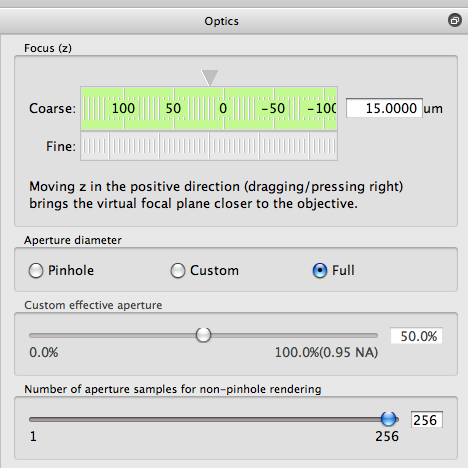
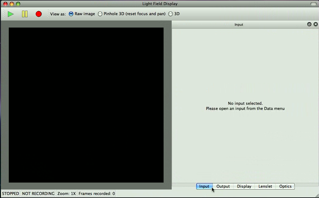
   Your screen should look somewhat like the screen in Figure 2.1. You should see five tabs labeled ``Input'', ``Output'', ``Display'', ``Lenslet'' and ``Optics'', as well as a control bar that has play, pause and record buttons as well as a display mode selector. If any of these are missing, select ``View'' in the menu bar and enable them.

4. Select ``Raw image'' from the view mode selector on the toolbar.

   You should see a black square on screen. You can pan the square by dragging with the right mouse button (or control-drag with the left mouse button on Mac). You can zoom in and out by either using the scroll wheel on the mouse, two finger scroll on a Mac trackpad or by pressing Ctrl and + simultaneously or Ctrl and - simultaneously (Use the Command button on Mac instead of Ctrl).

5. Select ``QImaging camera'' from ``Open input'' under the ``Data'' menu.

   This connects LFDisplay to the camera. You should now see an image coming from the camera. If no camera is connected, or if all cameras are in use, LFDisplay will show an error message. Sometimes, if camera software did not close cleanly, a camera might be stuck in a ``used'' state. Please switch the camera off and on to see if that fixes it.

6. Click the ``Display'' tab to visit the display settings panel.

   There should be a row of tab selectors along the bottom of the panels.

7. Click the ``Reset gain, offset, gamma'' button to reset postprocessing display settings.

   Figure 2.2: This is the display panel after the ``Reset gain, offset, gamma'' button has been pressed. Automatic gain control should be off, gain and gamma should be at 1.0 and offset should be at 0.0.

   

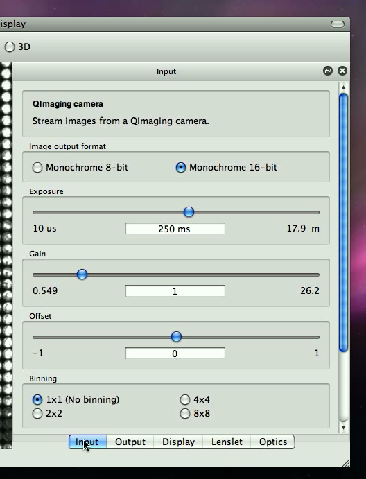
   This ensures that we get an accurate picture from the camera. Your display panel should look somewhat like what is shown in Figure 2.2.

8. Click the ``Input'' tab to visit camera settings (settings for the current input data source) and adjust the exposure (and optionally gain and offset) to achieve an image that does not saturate.

   Figure 2.3: This is the input panel for controlling camera settings. The exposure slider is the most important; gain and offset should be left at 1.0 and 0.0 if possible. You can scroll down to see some information about the current camera.

   

   Ideally, in order for the information captured to be correct, we want none of the pixels to be anywhere close to being at top brightness (white).

How do I calibrate LFDisplay for light field imaging?

1. Click the ``Optics'' tab to visit optical recipe settings.

2. Enter the microlens, objective and specimen information into this panel.

   Figure 2.4: The bottom portion of this panel allows the user to enter information about the optics being used in the light field microscope. This information will be needed to render the light field.

   

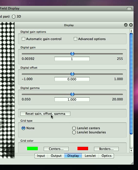
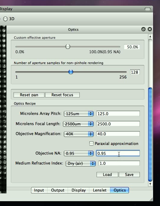
   You may need to scroll down to locate all the fields. LFDisplay needs information on the microlens array pitch, focal length, the current objective magnification, NA and the specimen index of refraction. If any values don't make sense, such as the NA exceeding the specimen index of refraction, the panel will warn you with the color red. Make sure ``Paraxial approximation'' is unchecked.

3. (Optional) Save these parameters using the ``Save'' button.

   You may wish to do so in order to quickly bring up parameters next time using the ``Load'' button.

4. Click the ``Lenslet'' tab, click ``Show rectification'', and click ``Reset'' in order to begin manual rectification.

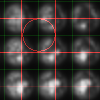
   You should see a green grid (lenslet centers) and a red grid (lenslet boundaries) overlaid on top of the camera image. The main idea here is to set the grid orientation and size such that the circles in the raw light field image are neatly contained inside one red box, with green crosshairs through their middle.

   Generally, the microlens array may not be perfectly aligned to the imaging system, so some amount of manual rectification is required. Furthermore, bumping the light field microscope setup may jitter the camera with respect to the microlens array. In these cases, readjustment of these values may be necessary, but a ``Reset'' isn't necessary.

5. Drag with the right mouse button (or Ctrl-drag the primary mouse button on Mac) until you can see the center (red) circle clearly.

   Figure 2.5: This is what the lenslet grid should look like. The image in (a) shows the default gridding, and the image in (b) shows the correct rectification.

   (a)	(b)

   You may need to zoom in or zoom out to see the red circle clearly. The circle should be roughly the size shown in Figure 2.5.

6. Adjust the ``Center lenslet position'' settings to recenter the red circle on the nearest circle (lenslet image) in the raw light field image from the camera.

   For the number controls in this panel, you can either type in values, click the top/down buttons, or use the up/down keys. Mouse wheel scroll is also an option. Page up or page down will move these values faster, as well as Ctrl-scroll (Command-scroll on Mac).

7. Adjust the ``One lenslet to the right'' settings until the red box to the right of the circle neatly contains the adjacent lenslet image.

8. Drag the image to the left and follow the red grid to the right, adjusting the ``One lenslet to the right'' value as necessary to keep the lenslet images roughly inside the red boxes.

9. Drag the image to the left so that the right edge of the image is visible. Adjust the ``One lenslet to the right'' value so that the rightmost whole lenslet image is contained inside a red grid.

10. Drag the image so that the center lenslet circle is visible again and repeat steps 7-9 for the ``One lenslet down'' value, while dragging the image up and following the grid pattern down.

11. Save the lenslet configuration.

    Click on ``Save'' to save the lenslet configuration. The light field image has now been manually rectified. As a sanity check, inspect random parts of the image to see if the lenslet images are still inside the red grid boxes. Sometimes, with geometric distortion/field curvature, the registration/alignment may not work, so just get it close enough. Also, check to make sure the center lenslet image is neatly outlined by the red circle. This should be the case if the NA, magnification and microlens parameters were specified correctly. If the lenslet image is too small compared to the red circle, either the microlens array isn't at the correct focal distance from the camera focal plane, or there's an extra stop in the system somewhere.

    After all checks are done, we are now ready to explore the specimen.

How do I interactively explore a specimen?

1. Click ``Pinhole 3D (reset focus and pan)'' on the ``View as:'' mode selector on the toolbar.

   You should now see a pinhole image rendering of the scene. The depth of field will be much greater than the depth of field as seen through the eye piece.

2. Place the mouse cursor on top of the image and drag using the left mouse button.

   By dragging the left mouse button, we are ``panning'' the sequence. To be more precise, it is as if we are viewing the scene through a pinhole in the telecentric stop of the objective, and moving this pinhole around. This should give you a sense of the depth of the specimen.

3. (Optional) If the exposure is short enough, move the stage to locate various other parts of interest in the specimen, because this is a live display.

4. Click ``Optics'' to go back to the optics settings and click ``Reset pan'' to reset the panning.

5. (Optional) Scroll the panel to the top if the focus section isn't fully unobscured.

6. Click ``Full'' under ``Aperture diameter'' to place the light field rendering in full aperture mode.

   Now, we should be able to refocus on different depths in the scene. This is equivalent to opening up the aperture stop in the objective, as opposed to using a pinhole.

7. Drag one of the focus sliders slowly to refocus the image.

   If your graphics card isn't fast enough, reduce the number of aperture samples for non-pihole rendering.

8. Type in a number into the focus input box to the right of the sliders to go to a specific depth.

   Keep in mind that negative values means we're focusing further away from the objective (deeper into the specimen) and positive values means we're focusing closer to the objective (shallower parts of the specimen).

   Figure 2.6: Refocusing is accomplished by dragging the focus sliders or entering values manually. Crop (c) of the rendered light field is the specimen focused at the original focal plane, as can be seen by the settings in (a). Crop (d) is the same region, but focused at a different depth, specified by the new depth in (b).

   (a)	(b)
   (c)	(d)

How do I save and load image data in LFDisplay?

1. Click the ``Output'' tab to select the output panel.

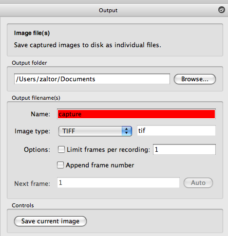
   Here we can save the raw image data from the camera so that we can explore these images later.

   Figure 2.7: This is the output panel, where we can capture either streams of images or take a single snapshot. The current filename is red because this file already exists and will be overwritten if we perform a capture.

   

2. Choose an output folder and choose an output name.

   The output name will turn red if the file already exists. Make sure the image type is ``TIFF''.

3. Click ``Save current image'' to record the current raw image to the file specified.

   Remember the filename and location, as we'll go back to it in a later step.

4. Enable the option ``Append frame number'' in the Output panel, click the record button (red circle) on the toolbar.

   This starts the movie recording mode of LFDisplay and appends a frame number to each recorded TIFF file.

5. Move the specimen around using the stage controls on the microscope.

6. Click the record button (red circle) to stop recording.

   Now that we have captured some images, we can view them in LFDisplay.

7. Select ``Single image file...'' in ``Open input'' under ``Data'' in the main menu. Select one of the files we captured to previously.

   Now, we can explore this specimen as captured at that specific time.

8. Explore the specimen by panning or refocusing as described previously.

   Note that none of the light field operations (panning/refocusing) are recorded. In fact, LFDisplay simply records raw frames from the camera in order to retain the most information from the scene. Remember to save lenslet rectifcation settings when recording files if you wish to revisit captured data later in LFDisplay.

9. Select ``Image file sequence...'' in ``Open input'' under ``Data'' in the main menu. Choose ``Create a new sequence from images'' and then select several of the files to load.

   This causes LFDisplay to display a light field movie looping continuously, simulating a live, animated scene.

10. Click ``Input'' on the list of tabs in order to bring up the input panel.

11. Change the frame rate to ``4''.

    Now, the animation should be playing at 4 frames per second.

12. Click the pause button in the toolbar.

    The animation should now be stopped.

13. Drag the frame number slider.

    This allows you to view a specific light field in the sequence.

14. Select a specific file in ``Image frames''.

15. Click either ``Move up'' or ``Move down'' to change its position in the sequence.

16. Click ``Add...'' and select some more files to add into this sequence.

17. Select one specific file and remove it from the frame list by clicking ``Remove''.

18. Save the information about which files are in this light field movie by clicking ``Save...''.

    You can load this information later to get a specific sequence of frames.

About this document ...

A Practical Introduction to
Light Field Microscopy

This document was generated using the LaTeX2HTML translator Version 2002-2-1 (1.71)

Copyright © 1993, 1994, 1995, 1996, Nikos Drakos, Computer Based Learning Unit, University of Leeds.
Copyright © 1997, 1998, 1999, Ross Moore, Mathematics Department, Macquarie University, Sydney.

The command line arguments were:
latex2html lfmintro.tex -split 0 -local_icons

The translation was initiated by Zhengyun Zhang on 2010-03-22