CS 348b Project
Pramod Kumar Sharma
Guillaume
Poncin
The idea in this project was to
render realistic pictures of a Christmas tree covered by snow at dusk.
The complex lighting due to the atmosphere and to the small lamps on
the tree, the modeling of pine trees and finally the modeling and
rendering of snow constitute the main challenges of this project.
1. Modeling snow
2. Modeling trees
3. Lights: glow effect
4. Global illumination using photon mapping
5. Subsurface scattering in snow
6. Miscellaneous...
Final images...
Proposal...
1. Modeling Snow
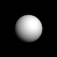
Show is modeled using metaballs. A metaballs is
described as an "isosurface," a surface that is defined by checking for
a constant value throughout a region in 3D space. In general metaballs
can have any kind of basic components but for modeling snow we used
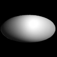
only spheres and ellipsoids. Following images
demonstrate the process of metaball generations using LRT:
Sphere
Ellipsoid
Blob with 2
ellisoids
Blob
with 4 ellipsoids
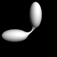
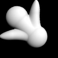
And finally an interesting one:)

The basic implementation of intersections with this primitive use the
ideas developed in Persistance of Vision (POVray). We extended it by
integrating a kdtree acceleration structure in the blob class for
speeding up the intersections when there are many components. This
resulted in a speed improvement from 20 min to 3 minutes of rendering
time for a blob with 20000 components.
Snow modeling using Metaballs:
To simulate the snow on various objects in the scene we thought
of using the ray tracer itself. Snow is considered as a ray coming from
some point at infinity with direction determined by gravity and winds.
So snow fall is basically a set of parallel rays intersecting
the scene. This framework allows to simulate snow coming from any
direction and we can put the snow on any kind of object. We can easily
control the size/density of snow.
To give a more realistic impression, we are
modulating the sphere into a rotated ellipsoid to better model the
aggregation of real flakes.
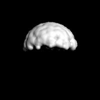
Following example demonstrate the idea where snow is projected on
a sphere from above. Figure shows only snow part.
Snow on
sphere
Layered Snow Fall: To get the realistic
feeling of now we did 2 layer snow projection upper layer having
smaller flakes. First layer with big blob element size represent the
shape of the object on which ray is projected and second layer present
finer details of snow flakes. This reduces number of blob elements
required to model snow on a given surface by a large amount. We did not
include this in our final scene since we could not get the expected
effect, unless we used too many blob components.
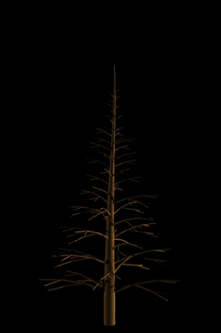
2. Modeling Trees:
We really wanted to have
realistic looking trees as the base for our image. We created an
L-system parser specialized for pine trees, as described by A.
Lindenmeyer. It is based on the parsing code written by N. Lambert
(Stanford PhD student). We extended his code to account for gravity and
to properly model the geometry of a cone-shaped tree. The rules for the
main tree are the following:
Axiom: \(100)O(0)D
O(t) : (t<=3) ==> ASASASASO(t+1)
S ==> L(0.9)!(0.85)+(0.5)
A ==>
E[&L(0.85)!(0.45)B]\(81)[Z&L(0.8)!(0.4)B]\(75)[&L(0.85)!(0.45)B]\(74)[Z&L(0.8)!(0.5)B]\(78)[&L(0.75)!(0.4)B]\(75)
B ==> YF[-L(0.8)!(0.9)WC]L!(0.9)C
C ==> YF[+L(0.8)!(0.9)WB]L!(0.9)B
The main difficulties that we
encountered in the modeling were to find this formula and to make the
needles look nice. The rules we use are very simple: O accounts for the
trunk, S for the transformations that occur along the trunk, A for the
main branch structures, B&C, that recursively call each other for
the small branches. The non standard symbols Y and W account for
gravity.
The needles are modeled by
elongated ellipsoids. They are pointing with a relative direction of 30
degrees with respect to the branches (omitting the gravity effect), and
disposed randomly along the branches. Their size vary as a function of
their position in the tree.
We roughly have 10000 objects
per tree (5% branches, 95% needles).
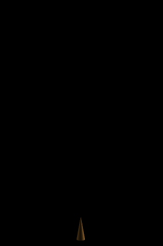
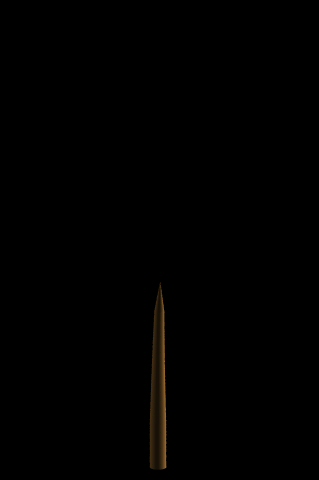
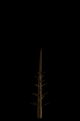
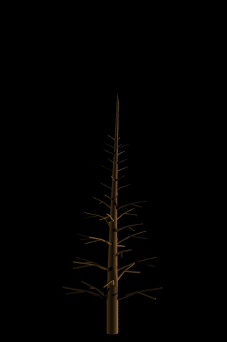
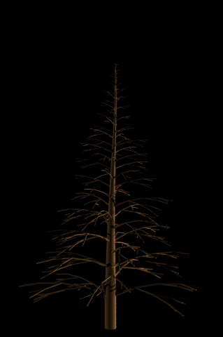
6 stages in the L-parsing of the
tree:
And finally, with needles:
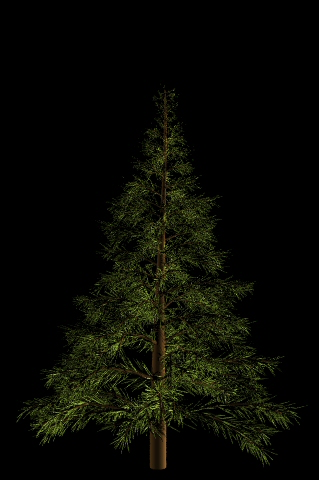
After we made our first tree, it was easy to
create a new model for each of the trees in the picture, by tweaking
the parameters slightly.
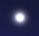
3. Glowing lights:
How can we integrate so many
lights in the scene without taking too much computation time ? We have
approximately 150 lights in the main tree and one in the moon. Using
area lights would have been suicidal, so we opted for point lights with
a nice camera-glowing effect.
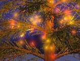
The glow is an approximation of
both the atmospheric effect and the spread of the light on the camera
film. The idea is to take the intersection of a ray from the camera
with the plane of the light source and to compute the distance between
this intersection and the light source. We use an exponential falloff
formula on the intensity of the light.
The main issue here was to get
the right parameters, so that the glow was not too weak or too strong,
allowing for all the other lights in the scene. We also spent some time
optimizing it since the distance computation has to be made for every
point in the scene multiplied by every glowing light.
4. Global illumination:
Finally, to get the soft feeling
of lighting from the scattering atmosphere, we implemented photon
mapping. The problem here was computation time. We put a lot of effort
into optimizing this part.
First, we implemented H.
Christensen's technique of irradiance precomputation. It speeds up the
final gathering step by a factor of ten.
Then we limited the sampling of
photons to the snow surfaces, as needles and branches would not account
for much of the diffuse lighting anyways. In order to get photons from
the sky, we treat it as a light source infinitely far from the scene
that emits low intensity light from every position on the hemisphere.
Final gathering rays that go to infinity are given the color of the
sky. That is how we get the blue coloration of the whole scene.
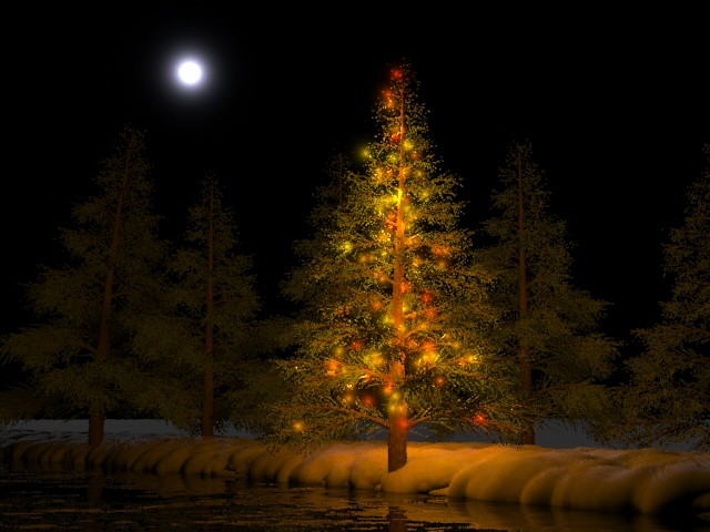
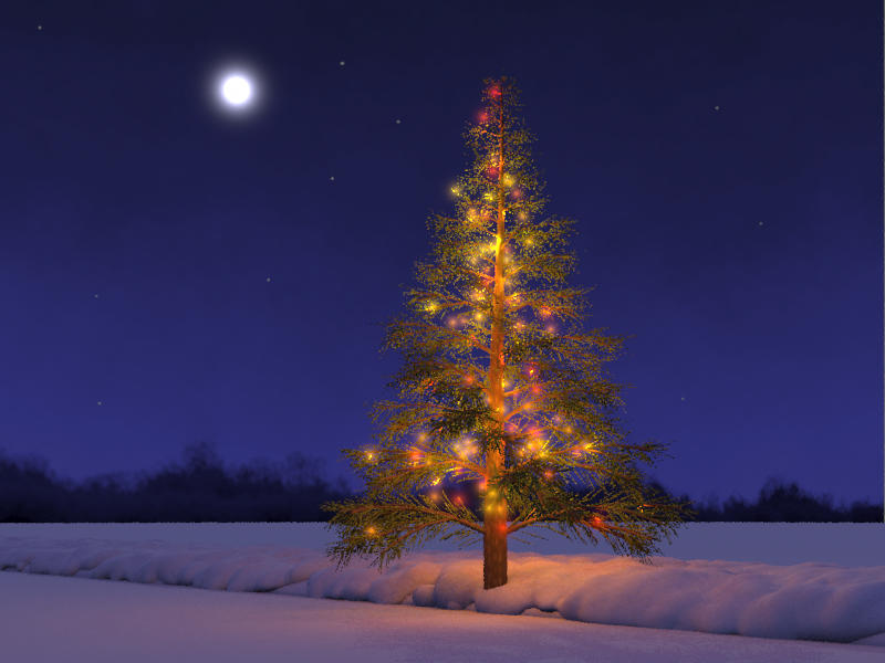
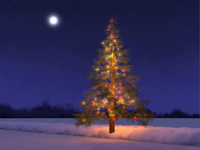
Without global illumination (and
no snow on the trees):
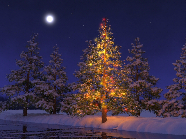
With global illumination:
5. Subsurface Scattering of snow:
Subsurface scattering to model
the translucency of snow is motivated from the Jenson's paper "A Rapid
Hierarchical Rendering Technique for Translucent Materials".
Implementing this method for snow gives couple of interesting
challenges:
Sampling the metaballs:
Uniform sampling the area of metaballs is itself a challenging problem.
We devised a simple sampling algorithm that works as follows:
For each sphere (or ellipsoid) in the blob we
generate rays originating from the sphere center and having uniformly
distributed direction in the sphere. The intersection points of these
rays with the blob that lies within the sphere are calculated. Then
these points are checked against the sample points on blob from the
neighboring spheres. Those sample points which are at a distance
less then some threshold from any of the neighboring sample
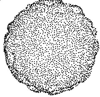
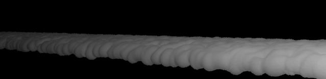
points are rejected. Following picture show the sampling points for
"snow on sphere picture" (top view)
Another issue with sampling was "how to make sure that it is
uniform and all the samples points have distance less than lu as needed
for the implementation of subsurface scattering". We did testing using
finding mean min-distance and variation to quantize the non-uniformity
of sampling.
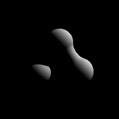
Following example shows one example which we generated from our
implementation of Jensen's paper. There are two light sources in the
scene. First light source is on the side and other is a red light in
the back side of scene.
|
A blob without Translucency
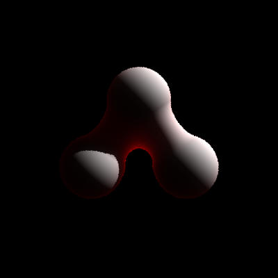
|
With Translucency
|
|
|
|
Snow without translucency
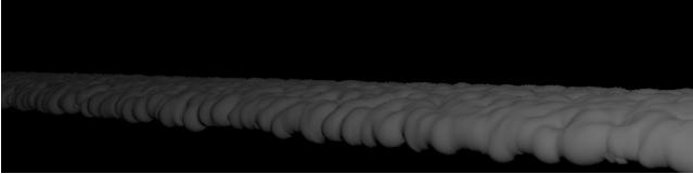
Snow with translucency
Snow without subsurface scattering
Snow with subsurface scattering
6. Miscellaneous:
There are many other details in the picture that
we worked on. We are just mentioning a few here...
Textures
First, we have icy water texture on the
foreground based on a very hacked version of the windy displacement
mapping in LRT. It is projected on a simple polygon, and gives the
right impression of half-frozen liquid element. We also have
cylindrical mapping of a procedurally generated texture on the trees
and a procedurally generated background for the sky (applied as a
texture).
Acceleration
We used the KdTree acceleration structure from LRT
but we had to modify it to make it work on the scene. The main issue is
that we have very large objects (quasi infinite plane, moon), and at
the same time very small details (needles). That is why we create one
Kd-Tree per group of shapes that belong to the same object. We end up
with 20 of these Kd-Trees, that we put into a top level Kd-Tree.
Final
images...
BACK