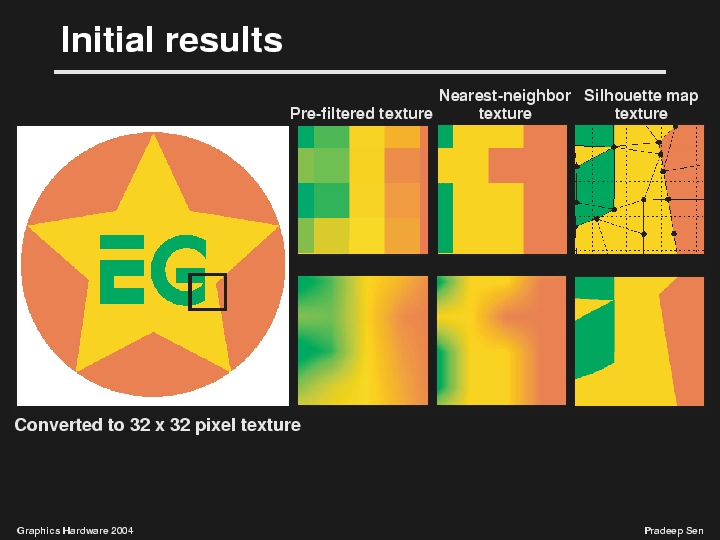
The vector graphics image shown on the left was converted to a texture 32x32 pixels in size. The black square indicates a region approximately 4x4 pixels big in the texture.
If we filtered the image when down-sampling it by averaging the region under each texel, we would get a texture as shown in the first column. This is normally how large textures or artwork is downsampled to reduce aliasing. Now if we bilinearly interpolate that when magnifying it we get something as is shown in left-most image in the bottom row. You can see that the texture is extremely blurry.
If we choose, instead, to perform a nearest neighbor sampling when downsampling the texture, we get something as shown at the top of the middle column. You can see the colors have not been mixed, but it has a pixelated appearance. A bilinear filtering of that texture is shown below it. Still, not acceptable.
Finally, if we use the silhouette map algorithm we propose in this paper, we see the results in the third column. The top image shows how the silhouette points define the discontinuities in the 32x32 silhouette map. You can see how the texture's cells are being deformed to match the edges of the G and of the star.
The final reconstruction using a silhouette map texture is shown below that. You can see how this accurately models the magnification of the original artwork.