The main focus of our final rendering project was an implementation of the "photon mapping" method developed by Henrik Wann Jensen.  We tackled photon mapping as a 2 step process:  in the first step, a large number (tens- to hundreds-of-thousands) of photons are emitted from all light sources, and these photons are traced through the scene.  Photons continue to bounce around the scene until they hit diffuse surfaces, at which point they are stored in the photon map data structure, or may continue to bounce around according to a certain probability distribution, contributing to indirect illumination.  The second step consists of ray-tracing the image and using the photon maps to compute estimates of the radiance at points where rays from the eye intersect the scene.

It is important to distinguish between the 3 different types of photon maps we build: the Global photon map, the Caustic photon map, and the Indirect photon map.  We use 3 separate photon maps to increase the efficiency of lookups in the already efficient kd-tree data structure that stores the positions of photon hits.  Each of these photon maps may be used separately in the rendering pass to estimate the radiance at points in the scene.  The power of each photon in the global and indirect maps is equal to the intensity of the light source divided by the total number of photons, which implies a conservation of energy in the scene.

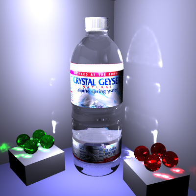
In addition to an implementation of photon mapping, our scene comprises of elements of bump mapping, texture mapping, and modeling in Maya 3 with heavy modification to the exported Renderman RIB files.  We used a public implementation of a kd-tree developed for scientific research to allow us to focus on more interesting issues related to rendering our scene.
 

A Reference Image for Test Scenes

Most of the effects possible with the photon mapping method are not possible in traditional Whitted style ray tracing.  Below is a reference image for some example images that follow and that highlight the effects possible with our photon maps.

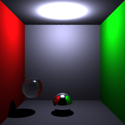
Traditional recursive ray traced image.  Notice how no light is focused through the glass sphere and none is reflected off of the metallic sphere.

Building the Global Photon Map

In building the global photon map, the photons are emitted equally in all directions from the light sources, and a portion of them are stored at the first diffuse surface they hit according to a probability of photons being absorbed or reflected.  Only photons that are absorbed are stored, and others are rejected in this pass.  This photon map can be used to simulate direct illumination, although we chose to disable it in our scenes.

Building the Caustic Photon Map

In building the caustic photon map, photons are emitted only in the direction of objects in the scene that are capable of producing caustic effects (ie specular and transmissive surfaces such as a shiny metal surface or glass surface).  We added a property to all primitives in the shading.h file called "generatesCaustics," which is true for the aforementioned types of surfaces and false otherwise.  In the scene.cc module, we build various vectors with information pertaining to these caustic primitives.  We create a list of these special primitives, a list of bounding spheres for these primitives, and a list of normalized probabilities for sampling each primitive based on the radius of the bounding sphere.  Bounding spheres are simply created from the bounding boxes of the objects, which isn't guaranteed to be so tight, but we make the slight optimization that spheres get their own tight bounding sphere.

As the caustic photon map is generated, it picks a random sphere based on the weights previously computed, and picks a random direction to sample the object within that sphere.  The caustic photon is sent out until it hits the caustic object within the sphere, and then is sent along its way until it hits a diffuse surface, at which point it is stored in the caustic photon map.  Contributions to the power of the photon may be modified by the medium with which it interacts, which resulted in nice colored caustics in our bottle scene.

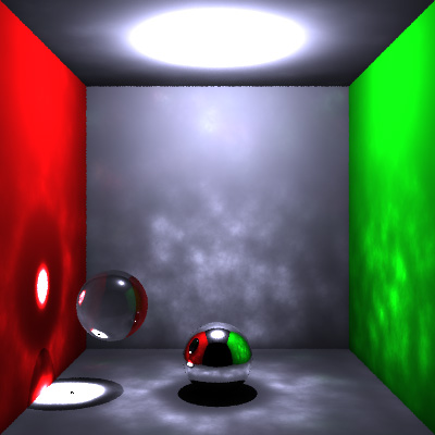
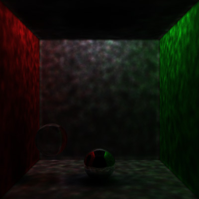
Below is an image of only the caustic photon map visualized in a simple box test scene.  Notice how light is focused through the glass sphere and is reflected off the metallic one.  Notice also how light bounces off the metallic sphere and is focused on the left wall.  The top wall is dark because we are visualizing only the caustic effects in this scene.  Note the "patchiness" of some of the caustics-- this is due to some roughness in the surfaces but can become smoother as more and more caustic photons are used in both the map and the estimate.

Larger: [800x800]  [1024x1024]
 

Building the Indirect Photon Map

Building the Indirect photon map is similar to building the global photon map, except that photons that hit diffuse surfaces have a certain probability of being reflected and continuing on their way.  The indirect photon map is used to simulate global illumination, in which colored surfaces may "bleed" color on other surfaces close by.  In the photon map construction pass, the number of global photons and indirect photons emitted should be equivalent (we used around 500,000 total for our scenes that best demonstrate the color bleeding). Since only a portion of these photons will be stored in the global photon map construction and only a portion will be stored in the indirect pass according to a certain probability, the portions should correspond to the probability function used for absorption/reflection.  For example, we saw numbers like ~70% absorbed on the first hit and stored in the global map, and ~30% reflected and stored in the indirect map.

Below is an image of only the indirect photon map visualized in the box scene.  Notice the way color bleeds off the side walls onto the white walls.  This is not possible in standard ray tracing.

Larger: [800x800]
 

The Rendering Pass

In the rendering pass, the photon maps are used at the point of interest to estimate the radiance at that point.  This is done as a sum over N number of photons, such that the contribution of a single photon is the brdf of the surface (calculated using the incoming direction of the photon) times the power of the selected photon.  This whole sum is then divided by the area of the projected sphere encompassing these N photons (a circle), and thus calculates the flux at that point.  We also applied a cone filter as described in Jensen's paper, although we discovered late in the process that the cone filter was actually introducing artifacts rather than helping-- when the photons were spread a little thin, the radiance estimates were not very smooth.  Using too low a number of photons could also result in estimates that were not very smooth.

The rendering pass basically adds the power of our photon maps to a whitted style integrator (we chose to implement only point light sources).  Although the global photon map worked, we chose to use the direct illumination model (sample the light) as an accurate estimation of direct illumination rather than the inaccurate and slower global photon map estimate, mainly because our focus was on caustics and the added rendering time was not warranted.  One nice optimization we made to the rendering pass was being able to distinguish when estimating radiance from the photon map would be a waste of time.  We did this by testing how far away the closest photon was from the current point of interest, and if it was above some threshold then no estimate was taken from the photon maps.

Rendering speeds were very good.  The 800x800 bottle image was rendered in about 30 mins on a 750 Mhz PC running Linux.  Besides obvious factors like image size and the number of pixel samples (we used 4 samples per pixel), rendering times were very dependent upon the number of photons used in the scene.  Building the photon maps never took more than about 2-3 minutes.  For some images like an 800x800 box scene with 120,000 caustic photons and 70 photons in the radiance estimate, rendering time was around 1 hour or more, and for the 1024x1024 images it was 2 hours or more.

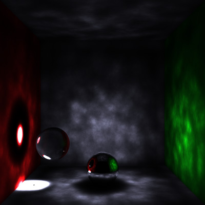
Below is an image that incorporates direct lighting, caustic effects using photon maps, and indirect lighting using photon maps (although it is low for this scene).  Compare it to the classic ray traced image on the right.
 

Larger: [800x800]
 

Animation!

We also produced a short animation of balls with caustic effects bouncing around in a box:

[http://www.stanford.edu/~huatchye/bouncingspheres.mov]
 
 

Additional Effects

In addition to our implementation of photon mapping, other effects present in our scenes are bump mapping and texture mapping.  Texture mapping was basically fully functional in LRT, but we did make good use of it by adding labels on the inside of the bottle with backward, lightened text and images to simulate being able to see through the other side of the labels.  Bump mapping was used on the labels to simulate a nice wrinkled effect, and also on the cap to simulate the vertical grooves present in the original.  To implement bump mapping we basically bind an image to a surface and use the RGB values as perturbed surface normal directions.

The bottle itself was modeled in Maya 3 and exported to Renderman RIB format (special thanks to Ronny Kim for help with Maya).  Editing the RIB file turned out to be a long and painful process, but we were pleased with the results.  Here's a nice picture that highlights the bump mapping:

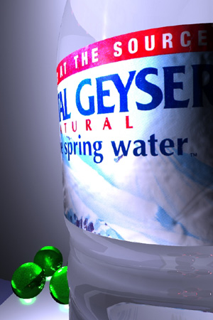
Larger: [493x740]
 
 

References

1.  Jensen, Henrik Wann.  "Global Illumination using Photon Maps" from Rendering Techniques '96 (Proceedings of the Seventh Eurographics Workshop on Rendering), pages 21-30, 1996.
2.  Jensen, Henrik Wann.  "A Practical Guide to Global Illumination Using Photon Mapping"  Siggraph 2001 course 38.
 

Copyright 2001 Zak Middleton

Feedback?
zacharym@stanford.edu