- Highly Optimized Kdtree
- Volume and Photon Mapping
- Volume scattering Importance sampling
- Almost no ray marching: cylindric lookups
- Irradiance caching
- PhotonMap based Importance Sampling for final gathering
- Irradiance gradient (rotationnal only)
Description of modeling attempts for the canyon
Looking closely to the pictures from Antelope canyon, one can see
that the walls are made up piecewise...
The erosion seems to have mostly
smoothed the wall surfaces, but we can see several sharp edges (mostly
vertically), indicating a change in the way the wall was eroded. Furthermore,
the texture left on the wall clearly shows the rock is made up of thin layers,
for the main part horizontal but that have been tilted and distorted in some
weird ways.
So the idea was to catch that composition of the walls, by
trying to decompose the scene into "rock" volumes and "empty" volumes. The
constraints on that separation should be that each rock volume has its own 3D
texture; that its frontier with an empty surface is smooth; and that the
junction between that frontier and those of its neighbors should be continuous,
but with discontinuity in the normal.
The idea we wanted to explore was
to model these blocks by
An aborted approach : 3D Voronoi diagram
We first thought about a 3D Voronoi diagram, as a rough estimation of the
repartition of our volumes. Casting a bunch of control points of type "empty"
and "rock" in the scene, that gives a partition of the 3D space in too
half-spaces : points closest to a "rock" control point would belong to the
canyon walls, and points closest to an "empty" rock would belong to the air
beind the walls. The problem with that approach you end up with walls
constituted of polygonal meshes, wich is not the aspect we expect. We did no
find a way to smoothe these walls, without losing the sharp edges at some point.
The potential we were trying to define was a weighted sum of potentials,
the potential at each control point being defined by the inverse of exponential
of the distance from the control point studied to the point in space we want to
categorize. The exponential falloff guaranteed that the contours remained
approximately those given by the Voronoi diagram ; but such an approach did not
guarantee the continuity of our potential when going from one region of space to
another.
Second thought : CSG modeling (Mathieu & Clovis)
We still wanted to model our walls with implicit surfaces, but each implicit surface would no define a smooth surface of the walls, not considering edges. Intersection of such volumes with constructive solid geometry would give us the desired sharp edges we can see on the walls, which are not very numerous after all.So we needed to implement CSG modeling in PBRT, in order to define intersection of volumes. We actually wanted to define our "basic volumes" for CSG modeling as shapes, which are actually oriented surfaces and which are not always closed. But one family of shapes in PBRT for which it is easy to define an "inside" function is the shapes defined by quadratic equations, such as the sphere and the cylinder.
Obviously, a surface defined as an isopotential of some potential over space can be given an "inside" function very easily.
We wanted to be able to do CSG modeling with at least the following basic shapes :
- the sphere : all it needed was the 'inside' function, since the surface is already closed ;
- the cylinder : it had to be closed, adding base and bound disks below and above the revolution surface ;
- a box : a very basic shape, ie a cube, which was not in PBRT
The most basic implicit surface : a "blob" (Clovis)
First approach
For our implict surface model now, we wanted to define some potential function given a small set of control points. The idea was to define a potential looking like an electric potential generated by a set of ponctual points. The overall potential, given N points, would then be the sum for i from 1 to N of potential values Ei(P) of the potential created by control point Pi at the point of space P. The electric potential from a ponctual charge goes as cst_i / dist(P, Pi)².A "blob" is defined as a (positive) isosurface of such a potential :
Blob = { P in space | E(P) = SUM Pi(P) = cste }
So to exactly compute the potential at a given point in space, the polynom to solve is of degree 2N-2, which is not pretty handy. An idea was then to approximate the function 1/x² by a piecewise linear function in x². for each control point, then, the space would be divided into concentric spheres. Between each two such spheres, the potential from the considered control point is then a polynom of degree two in terms of the parameter t of the ray. Outside the outer sphere, the potential is approximated to zero.
Thus, when going through a ray, for each control point Pi, and for the set of concentric spheres Sij in between each the potential generated by Pi is defined by a quadratic expression in t, we compute the values tij1, tij2 giving an intersection point between the ray and the sphere Sij. We try spheres Sij from largest to smallest, in order to abort the computation as soon as we can. For tij1, if the ray is "entering" the sphere, we add the polynomial expression of the potential inside S_ij (and outside S_i(j-1)), substract the expression of the potential given from outer sphere Si(j+1), and try ; if we go out of the sphere, the reverse operation will be applied. The events tij are sorted in increasing order, along with the degree two polynomial expression when "crossing" the event. We first initialize our potential expression given the parameter t we start, with is tmin. Then, for each event tij, we compute whethever E(P(t))=cst has a solution or not. If yes, we are done ; if no, we proceed with the next event tij.
Actually, that method, though working, was not really practical, since the ray could end up being subdivided in N * (number_of_intervals_for_inv_dist2_approximation), with the number of subdivision intervals increasing with the wanted accuracy. That seemed not really scalable to what we wanted to do with blobs (having a lot of control points), so we had to rethink the way blobs were defined.
Second approach
In fact, the major caveat of the above definition of a ponctual potential is that it has infinite extent. Though physically very reasonable, it was not realistic to actually define our pont potential that way. So we wanted to have a potential with finite extent, decreasing as the inverse square root of the distance to the potential point at least ; and another constraint is that it should be expressed as an expression of the squared distance, since that squared distance can be expressed as a degree two polynomial in the parameter t of the ray, but the square root of that polynomial does not give a polynomial.We ended up rediscovering the definition Povrayactually uses : a polynom of degree four in t, defined with parameter d² = dist(P,Pi)² as : Ei(P) = Ei0 * (1 - d²/ri²)² if d < ri, and 0 otherwise, ri standing for the influence radius of the potential point Pi. We are forced to resort to a polynomial of degree 4 (a quartic), since we want the derivative of that function (i.e. the gradient, i.e. the normal of the surface when considering points of an isopotential surface) to be continuous in ri.
The algorithm to compute the intersection (given by parameter t) between the ray and a blob defined by such a potential works in the same manner as previously : detect and sort all 'events' ti where the potential changes of expression, i.e. when entering or leaving an influence zone ; then march all the ray and for each event, solve the quartic equation in t E(t) = cste defining the blob. The actual polynom to solve is in fact of degree two whenever the portion of the ray considered is inside a single influence zone, which will often be the case in practice, presumably.
It is to note that the iterative algorithm to find polynom roots in an interval is faster than the solving using general expressions involving two radicals for the roots of a degree 4 polynomial. Descartes rule and root isolation using Uspensky's method will incur less computation in our case.
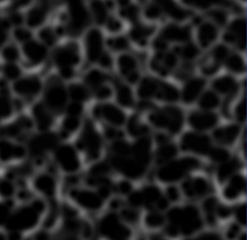
Here is what some basic blobs look like :
Actually, we defined our blob with some scaling along the axis, so that anisotropic potentials could be defined (i.e. elliptical blob elements). Blobs elements, as others basic shape elements, are defined in their local coordinated system, with the potential point being at the center, and the potential being isotropic. To compute the potential expression in t dued to a potential point, we compute the ray parameters in the blob element coordinate system, and retrieve the expression of the potential (which remains the same in any coordinate system) in that frame.
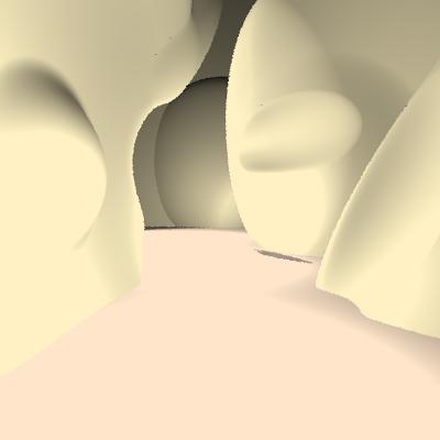
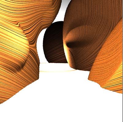
"Final" Result
Here is what we managed to model by hand with our very simple blob model for implicit surface. The result is not quite polished, and we actually did not try to plug CSG together with those blob shapes (laking of time for that). I actually spent much of my time modifying the potential expression for a single point, this modifying 3-4 times my shape code, and striving to make it robust (which in fact is not an easy task in ray tracing, much like for the problem we encountered with CSG), I lacked time to make anything satisfying for the modeling of the walls in the canyon. Here is the picture we got for the demo on Monday (we did not show it though, being a bit ashamed of it...) :
Dust And Sand (Mathieu)
I do not wanted the dust to have this weird homogeneous feeling, so I modeled a perlin noise volume density that with an Henyey-GreenStein Phase Function. This allows to control the amount of front and back scattering and at the same time is quite easy to importance-sample which will be required in the photon mapping algorithm.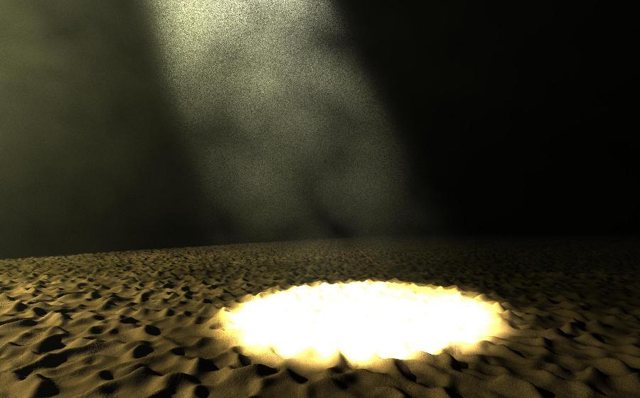
The sand is modeled with an improved version of the hw2 heightfield that can be tiled at infinity. This one is defined by a grayscale image I created in photoshop. I got rid of the seems by iteratively swapping the left/right and top/down parts and painting on the seems.
Texturing of walls (Clovis)
I did not have time to try any interesting texturing by the demo deadline, unfortunately. The idea, though, was to apply a 3D texture on each wall object of the scene.We though that the basic 3D texture would be a stack of thin layers of different color, in the brown tones mainly. After that, each object would have its own geological history, thus leading to a different configuration of the layers for each object. The layers needs to not follow exactly horizontal plane, so it has to be perturbed in some way, while trying to keep an overall constant orientation.
The method I just tried today (Wednesday, June 9th) is to put a plain brown texture, and to scale it by a number given position (x,y,z) of the point considered in object space. The scaling factor I used, in order to get a 1-dimensional noise, was actually just the FBm noise function applied in one space dimension (the x axis for instance), and given as a single coordinate parameter a function of (x,y,z) ; the value returned for the texture would be something like FBm( Point (f(x,y,z), 0, 0) ,
Here is the result I got. Unfortunately, we did not have time to fully wrap up that modeling with the photon mapping and importance sampling Mathieu implemented on his own side.
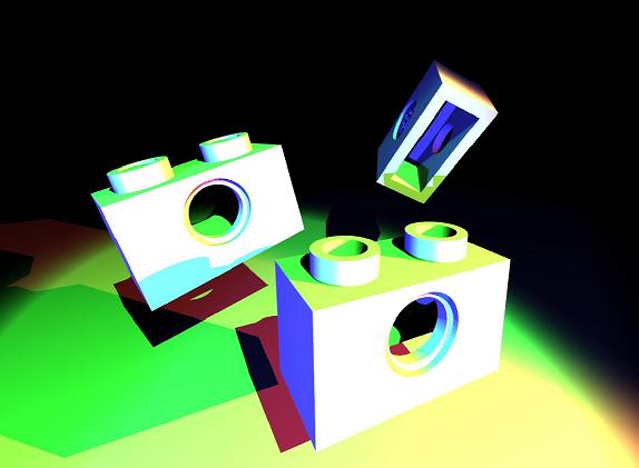
Lighting (Mathieu)
The main challenge in the scene we wanted to render is that the only direct illumintation part of the image is the light shaft (both its volume, and the surface of its base)
Highly Optimized Kdtree
The kdtree has been rewritten to produce maximum efficiency the memory footprint of its index is reduced to a single float per photon. The index is is stored in its depth first search order ather than in a heap-like order. This helps memory coherency. Finally the lookup are now iterative to be faster.Volume Photon Mapping
The volume photon mapping algorithm has been implemented in the guidelines of The "realistic image synthesis using photon mapping" book from HW Jensen. It uses russian roulette and importance sampling of the HG phase function. To reduce the artefacts, I implemented the volume and surface gaussian and cone filters. The Constants in [Jensen] of the gaussian filter do not normalize the gaussian filter by the way.Irradiance caching
It uses rotationnal Irradiance gradient (from Ward and Heckbert). These were easier to use than translationnal gradients because they are easy to evaluate whatever the underlying pdf. The irradiance cahcing algorithm features a photonmap based importance sampling of the final gathering step to compute the irradiance samples. This comes directly drom the paper "Importance sampling with Hemispherical Particle Footprints" from H Hey and W Purgathofer.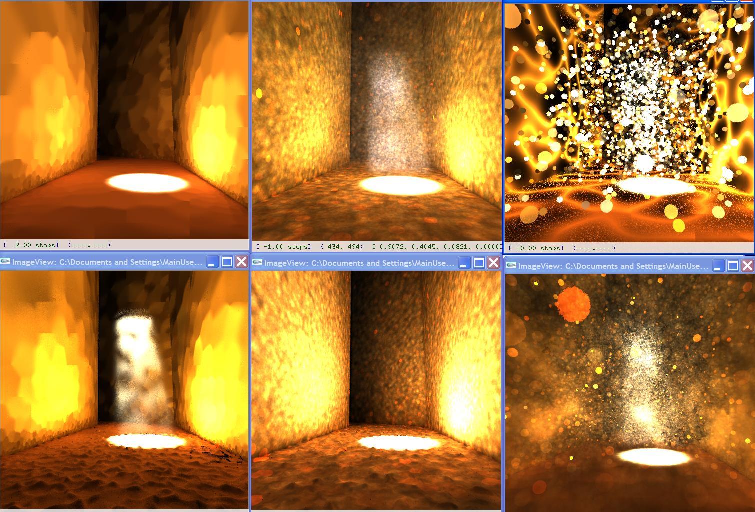
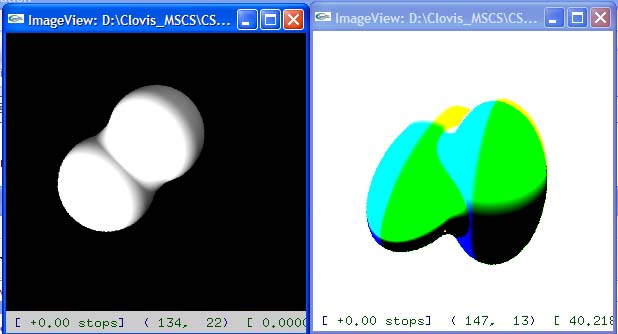
The left ones feature a coarse irradiance caching approximation, the middle ones are direct vizualisation of the photon map. The right ones are some of the many tests (too few volume photons above, cloud too dense below). I especially like the one above. I really do not know why this funky caustic effect has appeared!!
Main Contribution: Volume Photon Mapping Integration with cylinder look ups (Mathieu)
The way to compute multiple scattering is described in the literature, as follows:A spherical integral is evaluated at some given or adaptative time steps along the ray. This produces high frequency noise because the sampling is not equal along the ray and it is not efficient. If a high degree of accuracy is required, the time steps will be small and consecutive spherical lookups of the photon maps will be really correlated. If the direct lighting is done via the photon map, the ray marching is done via the cylindric lookup and not separately.
I figured out a way to sample this integral with much less variance in the same running time. This integral over te length of the ray and every direction can be computed using a cylinder-lookup of the photon map. The kd tree is queried with a cylinder instead of a sphere qhich will also decrease its radius is many photons were to be found. The cylinder is sliced between each photon and thus each photon is now a unique sample of a given slice of the cylinder. I thought about two ways to continue exploring this idea: first a viewing cone could be used instead of a cylinder to get some visual importance. The other idea is the opposite: to get a constant contribution per photons, the cylinder should rather be shrunk so that the transmission divided the radius squared is constant.
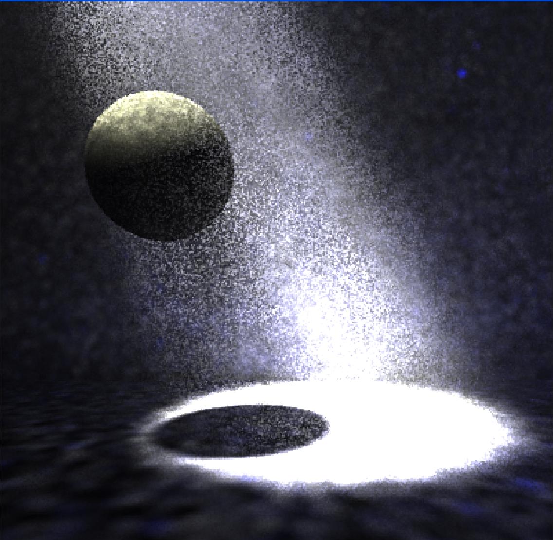

Here is the simple pbrt test scene, but here multiple scattering is
implemented via photonmapping. both image take roughly 100s to render. The left
one is the classic method that integrates over spheres at successive time steps.
The right one has the advantage of turning this high frequency noise into low
frequency. (the photon maps are here shown directly).