Reconstructing Occluded Surfaces using Synthetic Apertures:
Stereo, Focus and Robust Measures
This page shows detailed results from experiments 1 and 2 (described in section 4.1 and 4.2 of the paper).
Contents
Experiment 1: Synthetic Scene
To measure the performance of our cost functions (stereo, focus, median, entropy) under
varying amounts of occlusion, we experimented with a synthetic scene in which we can
control the amount of occlusion precisely. In this page, we describe the synthetic scene
(foreground occluder and background) we used, and the performance measurements of the
four cost functions (accuracy versus amount of occlusion).
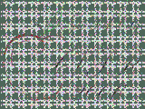
Our synthetic scene consisted of two frontoparallel planes, the foreground plane partially
occluding the background.

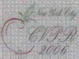
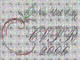
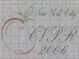
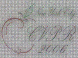
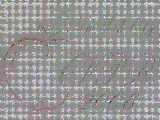
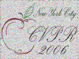
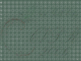
Background plane
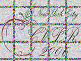
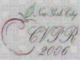
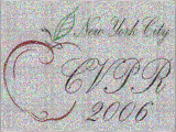
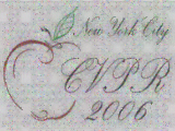
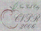
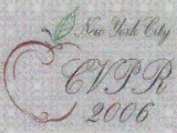
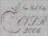
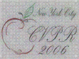
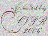
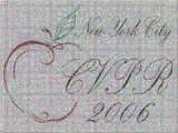
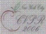
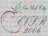
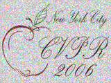
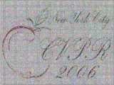
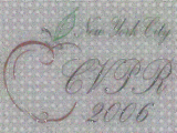
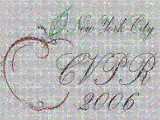
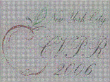
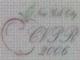
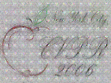
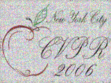
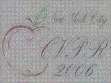
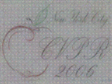
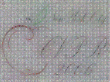
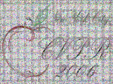
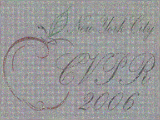
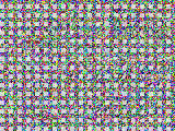
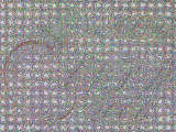
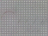
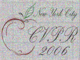
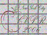
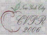
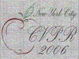
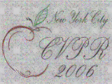
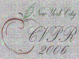
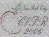
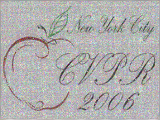
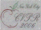
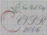
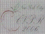
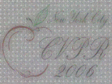
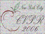
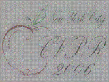
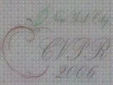
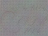
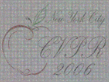
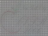
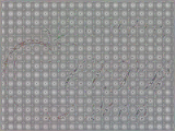
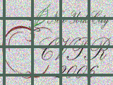
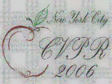
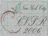
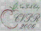
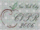
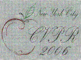
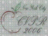
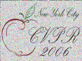
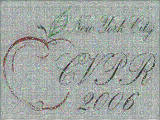
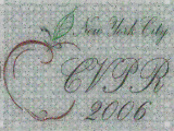
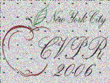
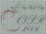
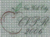
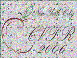
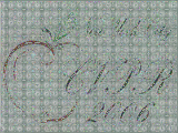
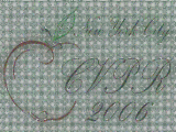
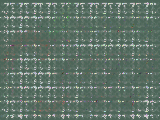
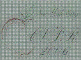
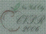
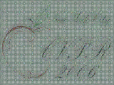
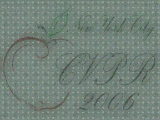
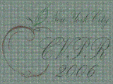
The background surface (which we seek to reconstruction under partial occlusion) was a plane
shown above. The texture on the plane is a composite of the CVPR 2006 logo (70%) and random
noise (30%). Noise texture was added to eliminate errors due to lack of texture, since our
goal here is to measure the errors due to occlusion.
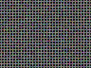
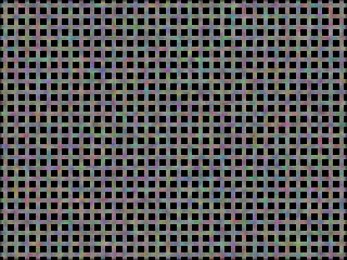
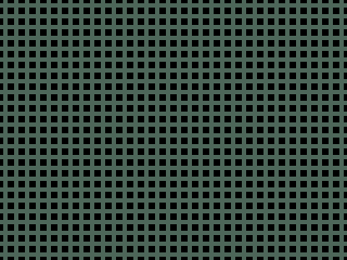
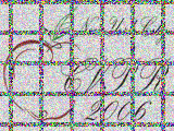
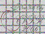
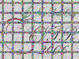
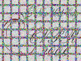
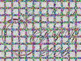
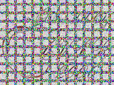
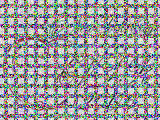
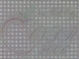
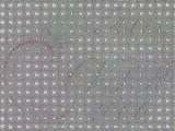
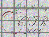
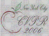
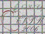
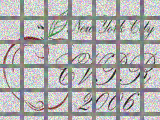
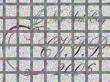
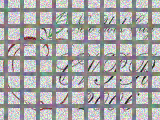
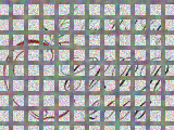
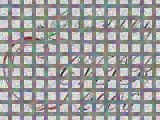
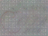
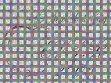
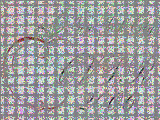
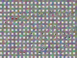
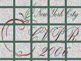
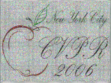
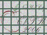
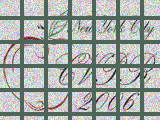
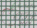
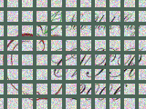
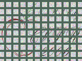
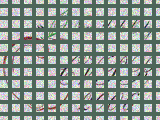
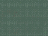
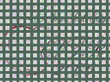
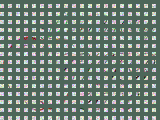
Foreground occluders used. By varying the spacing between the horizontal and vertical bars, we
can control the amount of occlusion. Here we show the spacing corresponding to 64% occlusion. We
used three kinds of textures for the foreground occluder: white noise (left), pink noise (center)
and uniform color (right).
We chose a trellisized foreground occluder consisting of horizontal and vertical bars as shown above.
The accuracy of reconstruction will depend on the amount of occlusion, as well as the texture on the
occluders. We control the amount of occlusion by varying the spacing between the bars, in our
simulation we used occluder density from 20% to 75%. We experimented with three kinds of textures
for the foreground occluder: white noise, pink noise (white noise convolved with a 5x5 box filter)
and textureless occluder (uniform color).
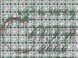
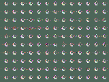
We used images from 81 views in our simulation. The cameras were on a plane looking at the background
layer through the foreground trellis. The camera positions were chosen by adding random offsets to
a 9x9 grid. It is important to use jittered camera positions rather than a regular grid since we are
using a regular grid of bars for the foreground occluder. If we placed our cameras on a regular grid,
we would get additional errors due to the strong correlation between visbility and camera positions.
This is a situation that rarely arises in practise, and would contaminate our simulation to measure
accuracy versus amount of occlusion.
The size of the synthetic aperture was chosen so that the horizontal disparity between the leftmost
and rightmost cameras was 40 pixels.
Here are the reconstructions obtained using the four cost functions, organized by the nature of
the texture on the foreground occluder.
| Mean Occluder density |
Image from central camera
| Reconstructed background using stereo (variance) |
Reconstructed background using median |
Reconstructed background using entropy |
Reconstructed background using focus |
| 19% |
 |
 |
 |
 |
 |
| 22% |
 |
 |
 |
 |
 |
| 27% |
 |
 |
 |
 |
 |
| 31% |
 |
 |
 |
 |
 |
| 36% |
 |
 |
 |
 |
 |
| 45% |
 |
 |
 |
 |
 |
| 49% |
 |
 |
 |
 |
 |
| 56% |
 |
 |
 |
 |
 |
| 64% |
 |
 |
 |
 |
 |
| 75% |
 |
 |
 |
 |
 |
To measure the accuracy of all four cost functions under varying
amounts of occlusion, we plot graphs showing the perectage of pixels
whose depth is correctly reconstructed (within one disparity level)
versus the amount of occlusions. The graphs for the different occluder
textures are listed below.
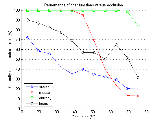
Occluder with white noise texture
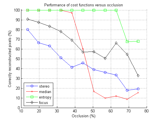
Occluder with pink noise texture
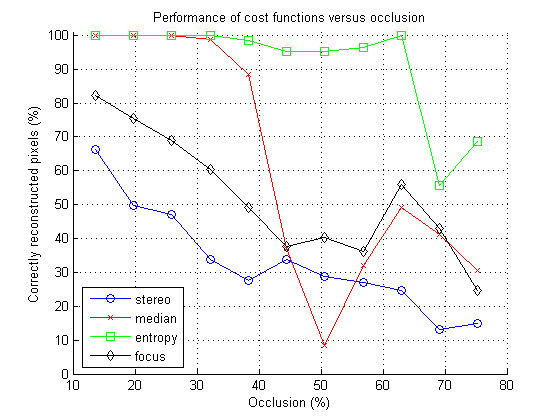
Textureless occluder (uniform color)
For clarity, we include EPS files for the graphs, viewable in any postscript viewer.
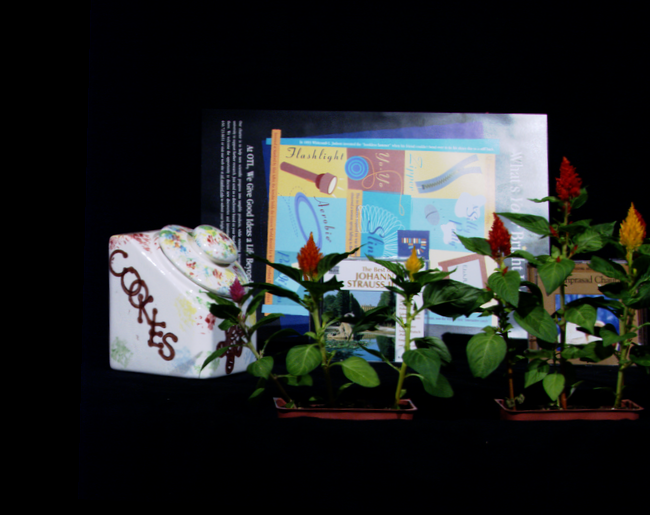
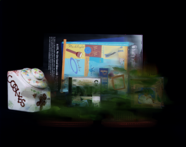
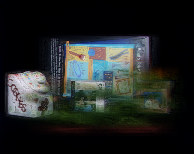
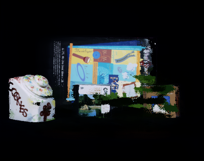
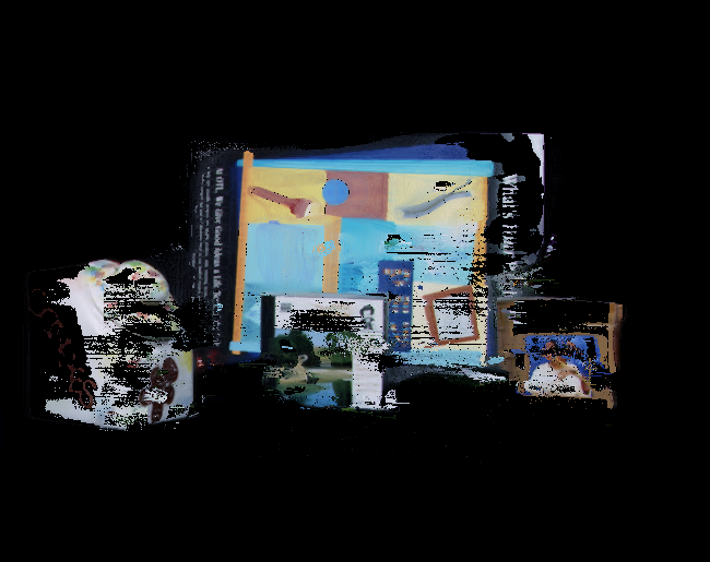
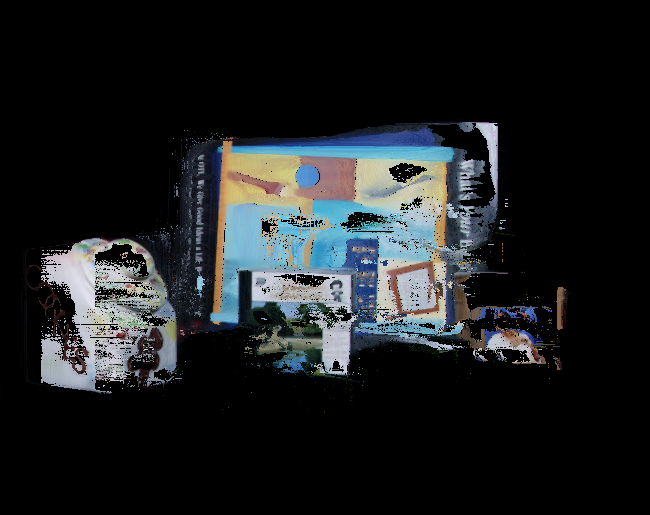
Experiment 2: CD Case behind Plants
We captured a 105 image light
field of a scene consisting of objects behind plants shown below. We compare the performance of the four methods introduced
in the paper - stereo, focus, median, entropy - as well as voxel coloring [Seitz and Dyer, CVPR 97] on reconstructing the
occluded objects in the scene.
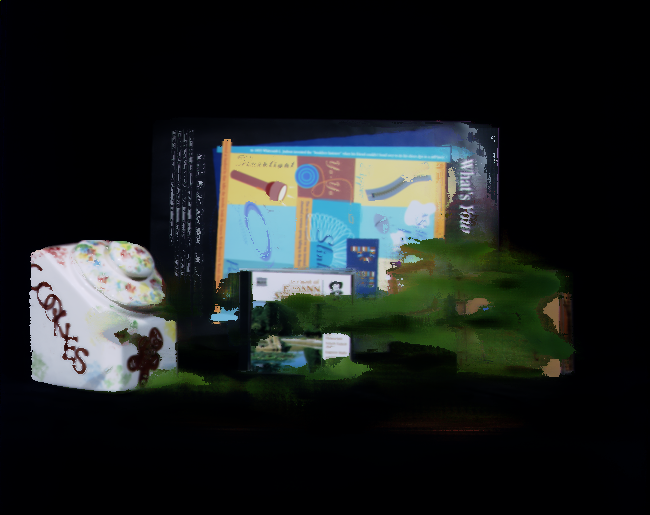
Our test light field consists of 105 images of a scene in a 21x5 grid.
This was acquired with a camera moving on a computer-controlled gantry. We acquired an identical light of the scene
with the plants removed. Here are the corresponding images. These are the gold standard for our experiments.
We are particularly interested in evaluating how well the different methods can reconstruct the Strauss CD case
in the center. (Please click on any of the images in this page to view them at full resolution).
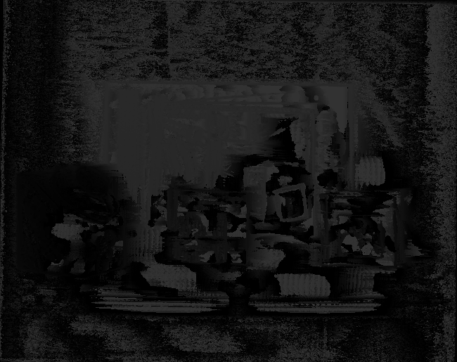
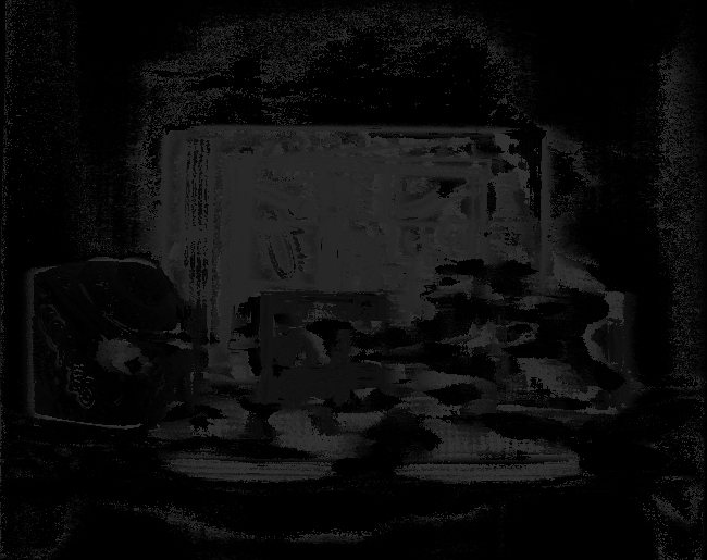
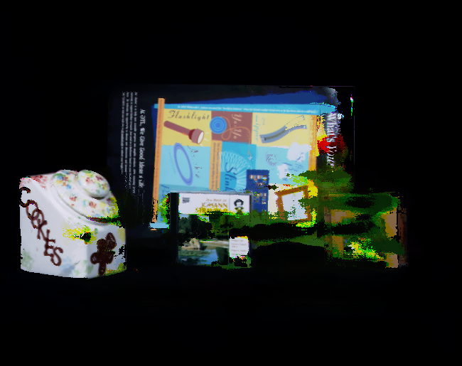
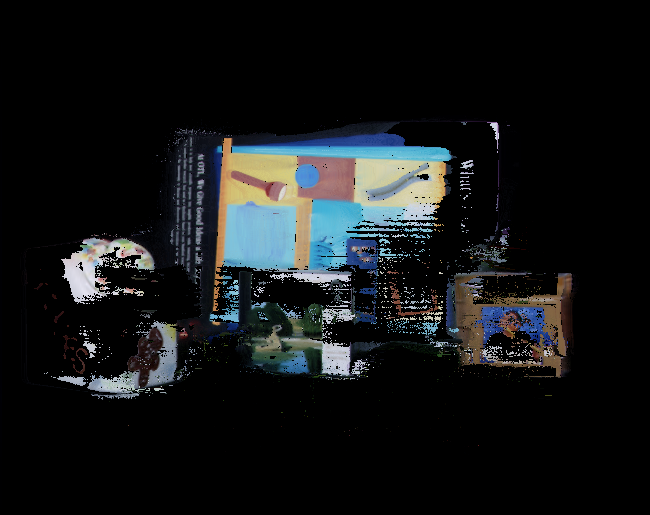
We computed depth maps and winner color images (defined in section 4, para 1) for each method, searching a range of
51 disparity levels behind the plants. The computed disparity maps, along with the winner color images are shown below.
| Cost Function |
Winner Color Image |
Disparity Map |
Stereo
(variance) |
 |
 |
| Focus |
 |
 |
Median
(component-wise) |
 |
 |
Entropy
(component-wise) |
 |
 |
Entropy
(color histogram) |
 |
 |
In component-wise entropy, we compute the entropy (and winner color) independently for each color channel. An alternative is
to divide the RGB color space into bins and compute entropy of a color histogram. This is shown in the last row.
We compare the above results with voxel coloring for a
range of thresholds. We used a voxel grid spanning a range of 161
disparity
levels, the last 51 of which are the same as those used in the
preceding section. After reconstructing the voxel grid, we delete
all voxels which lie in the first 110 depths, leaving only those voxels
behind the plants. These are projected into the central
camera, resulting in the images below.
Threshold = 20 |
Threshold = 25 |
Threshold = 30 |

Threshold = 35 |
Note that there is no single threshold value for which the scene (or even in the Strauss CD case in the center) are
reconstructed correctly.
Finally, we show comparisons between all pairs amongst stereo, focus, median, entropy on the reconstruction of the
Strauss CD case in the center of the scene. We have measured ground truth for this manually.

Image of CD case without plants
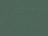
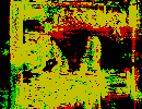
The chart below shows which points on the surface of the CD case were constructed correctly. Each image compares two methods.
Pixels reconstructed correctly (within one disparity level of ground truth) are colored
yellow, pixels not reconstructed by
either are colored black. Pixels reconstructed correctly only by the first method are colored red,
those reconstructed correctly only by the second are colored green.
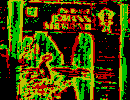
Focus vs Stereo |
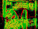
Focus vs Entropy |
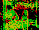
Focus vs Median |
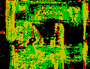
Stereo vs Entropy |

Stereo vs Median |
|
Entropy vs Median |
|
|
(Here entropy refers to component-wise entropy).