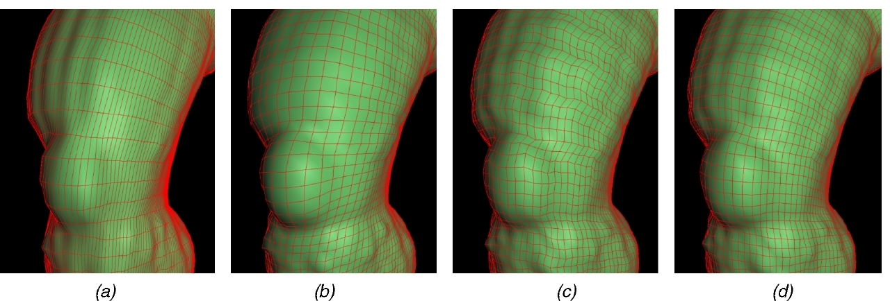
Caption for Figure 5:

This figure explores the three sampling criteria on part of the right leg of the model in figure 12a. Each of the above images represents a triangulated and smooth shaded spring mesh at a very low resolution. In each case, the number of spring points sampling the polygon mesh was kept the same. The differences arise from their redistribution over the surface. The spring edges are shown in red.

(a) shows what happens when the aspect ratio criterion is left out. Notice how a lot of detail is captured in the vertical direction, but not in the horizontal. (b) shows the effect of leaving out the arc length criterion. Notice how the kneecap looks slightly bloated and that detail above and around the knee region is missed. This is because few samples were distributed over the knee resulting in a bad sampling of this region. (c) shows a missing fairness criterion. The iso-curves exhibit many ``wiggles''. Finally (d) shows the result when all three criteria are met. See figure 8a for the original model and 8e for a full resampling of the leg.

Caption for 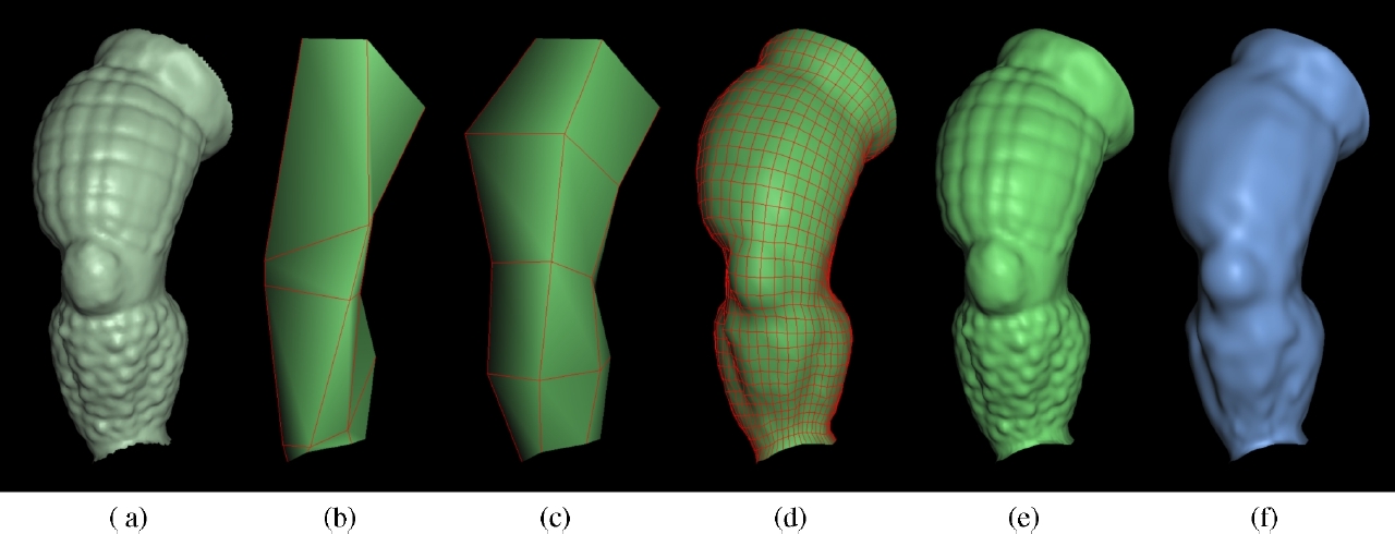figure 8:

The above represents a summary of our strategy for resampling a polygonal patch into a regular grid. (a) shows the original polygonal patch (the right leg from the model in figure 12a. This particular patch is cylindrical and has over 25000 vertices. (b), (c), (d) and (e)show a triangulated and smooth shaded reconstruction of the spring mesh at various stages of our re-sampling algorithm. We omit the lines from (e) to prevent clutter. (b) shows the initial guess for u and v iso-curves (under 4 seconds). Notice that the guess is of a poor quality. (c) shows the mesh after the first relaxation step (under 1 second). (d) shows the spring mesh at an intermediate stage, after a few relaxation and subdivision steps (under 3 seconds). (e) shows the final spring mesh without the spring iso-curves. Notice how the fine detail on the leg was accurately captured by the resampled grid. This resampling took 23 seconds. All times are on a 250 Mhz Mips R4400 processor. (f) shows a spline fit that captures the coarse geometry of the patch. This surface has 27x36 control points. It took under 1 second to perform a gridded data fit to the spring mesh of (e).

Caption for 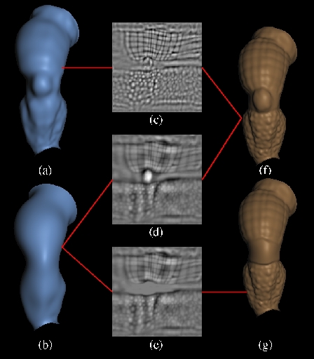figure 11:

This figure explores the possibility of multi-resolution editing of geometry using multiple displacement map images. All grayscale displacement images in this figure represent the normal component of their corresponding displacement maps. Displacement values are scaled such that a white pixel represents the maximum displacement and black, the minimum displacement. (a) shows a B-spline surface with 24x30 control points that has been fit to the patch from figure 8a. (c) is its corresponding displacement image. (b) shows a B-spline surface with 12x14 control points that was also fit to the same patch. Its displacement image is shown in (d). The combination of spline and displacement map in both cases reconstructs the same surface (i.e. the original spring mesh of figure8e). This surface is shown in (f). We observe that (c) and (d) encode different frequencies in the original mesh. For example (d) encodes a lot of the coarse geometry of the leg as part of the displacement image (for example the knee), while (c) encodes only the fine geometric detail, such as bumps and creases. As such, the two images allow editing of geometry at different scales. For example, one can edit the geometry of the knee using a simple paint program on (d). In this case, the resulting edited displacement map is shown in (e) and the result of applying this image to the spline of (b) gives us an armour plated knee that is shown in (g).

Operations such as these lead us to the issue of whether multiple levels of displacement map can essentially provide a image filter bank for geometry i.e. an alternative multi-resolution surface representation based on images. Note however that the images from (c) and (d) are offsets from different surfaces and the displacements are in different directions, so they cannot be combined using simple arithmetic operations.

Caption for 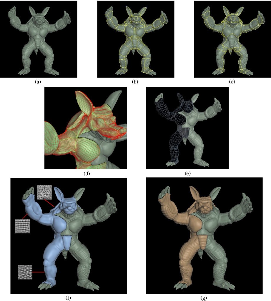figure 12:

Data fitting to a scanned model:

(a) is the polygonal model (over 350,000 polygons, 75 scans). (b) and (c) show two different sets of boundary curves painted on the model. Each was specified interactively in under 2 hours. The patch boundaries for (d), (e), (f) and (g) are taken from (b). (d) is a close up of the results of our gridded resampling algorithm at an intermediate stage. The spring mesh is reconstructed and rendered as triangles and the spring edges are shown as red lines. The right half of the figure is the original polygon mesh. (e) shows u and v iso-curves for all the fitted and stitched spline patches. (The control mesh resolution was chosen to be 8x8 for all the patches.) (f.) shows a split view of the B-spline surfaces smooth shaded on the left with the polygon mesh on the right. A few interesting displacement maps are shown alongside their corresponding patches. (g) shows a split view of the displacement mapped spline patches on the left with the polygon mesh on the right. Note that the fingers and toes of the model were not patched. This is because insufficient data was acquired in the crevices of those regions. This can be easily remedied by using extra scans or hole filling techniques. The total number of patches for (b and d through g) were 104 (only the left half have been shown here). The gridding stage took 8 minutes and the gridded fitting with 8x8 control meshes per patch, took under 10 seconds for the entire set of 104 patches. All timings are on a 250 Mhz MIPS R4400 processor.

Caption for figure 13:

Games one can play with displacement maps:

(a) shows a patch from the back of the model in 12a. The patch has over 25,000 vertices. We obtained a spline fit (in 30 seconds) with a 15x20 control mesh, shown in (b) and a corresponding vector displacement map. The normal component of the vector displacement map, is displayed as a grayscale image in (c). (d) and (e) show the corresponding displacement and bump mapped spline surface. The differences between (d) and (e) are evident at the silhouette edges. The second row of images show a selection of image processing games on the displacement map. (f) shows jpeg compression of the displacement image to a factor of 10 and (g) shows compression to a factor of 20. (h) represents a scaling of the displacement image, to enhance bumps. (i) demonstrates a compositing operation, where an image with some words was alpha composited with the displacement map. The result is an embossed effect for the lettering. Finally, the third row of images (j - l) show transferring of displacement maps between different objects. (j) is a relatively small polygonal model of a wolf's head (under 60,000 polygons). It was fit with 54 spline patches in under 4 minutes. The splined model is shown in (k). (l) shows a close up view of a partially splined result, where we have mapped the displacement map from (c) onto each of 4 spline patches around the eyes of the model.