Wavesolver Dataset
Supplemental Material for Paper: Toward Wave-based Sound Synthesis for Computer Animation
Introduction
Below we release scene information (geometry models, meshes), acoustic shader data (impulse files, input wav for speaker shaders, etc.), and the wavesolver configuration (cell size, time step size, etc.) accompanying our paper. Data format for each type of shaders (rigid-bodies, thin-shells, water, 3D re-recording and characters) are explained accordingly. If anything is unclear, please contact the paper authors for further clarification.
Click on the images ("Rendering") below for the full video!
| Name | Rendering | Solver snapshot | data | h | L | C | T | N | Runtime | N_t | alpha | x_l | N_c | eps_i |
|---|---|---|---|---|---|---|---|---|---|---|---|---|---|---|
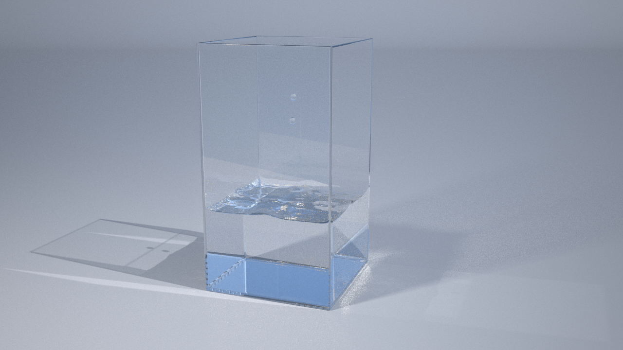
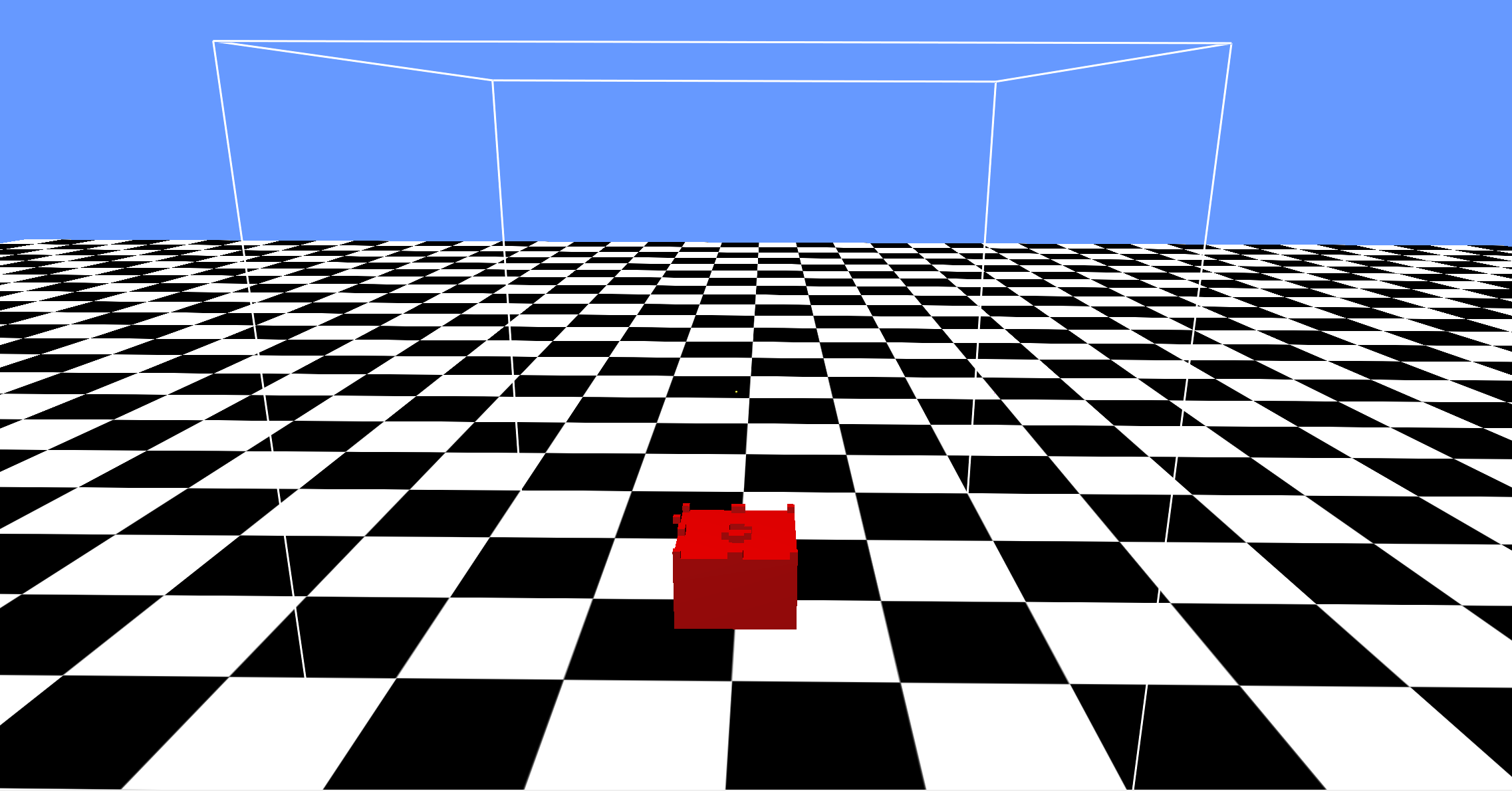
| Dripping Faucet (Water) |
 |
 |
zip (131MB) | 5 | 80 | (0.0,0.15,0.0) | 8.5 | 1600k | 18.6 hr | 32 | 2E-7 | (0.08,0.22,0.1) | 1 | N/A |
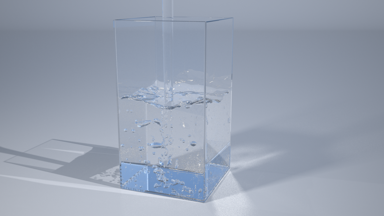
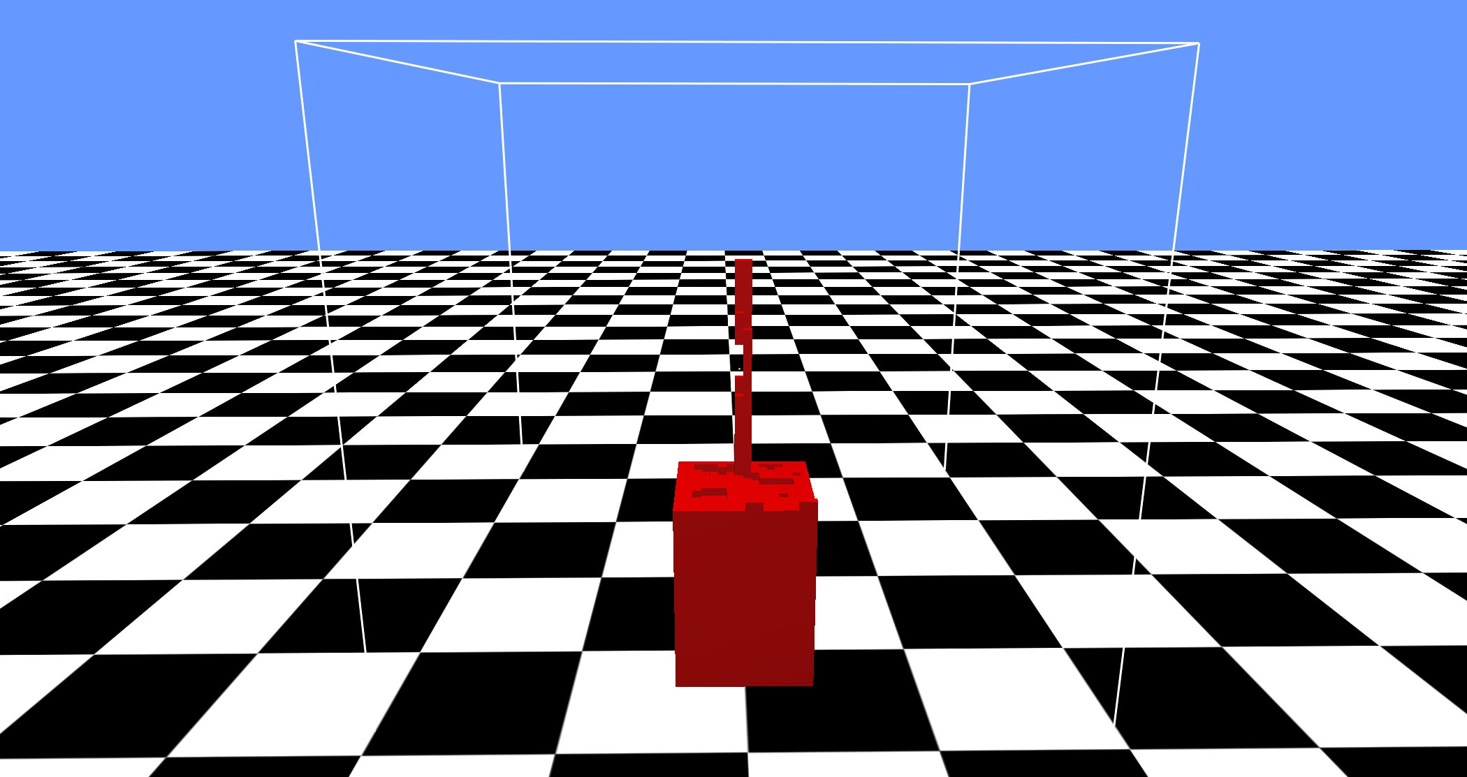
| Pouring Faucet (Water) |
 |
 |
zip (17GB) | 5 | 80 | (0.12,0.15,0.0) | 8.5 | 1600k | 55 hr | 64 | 2E-7 | (0.225,0.189,-0.0975) | 1 | N/A |
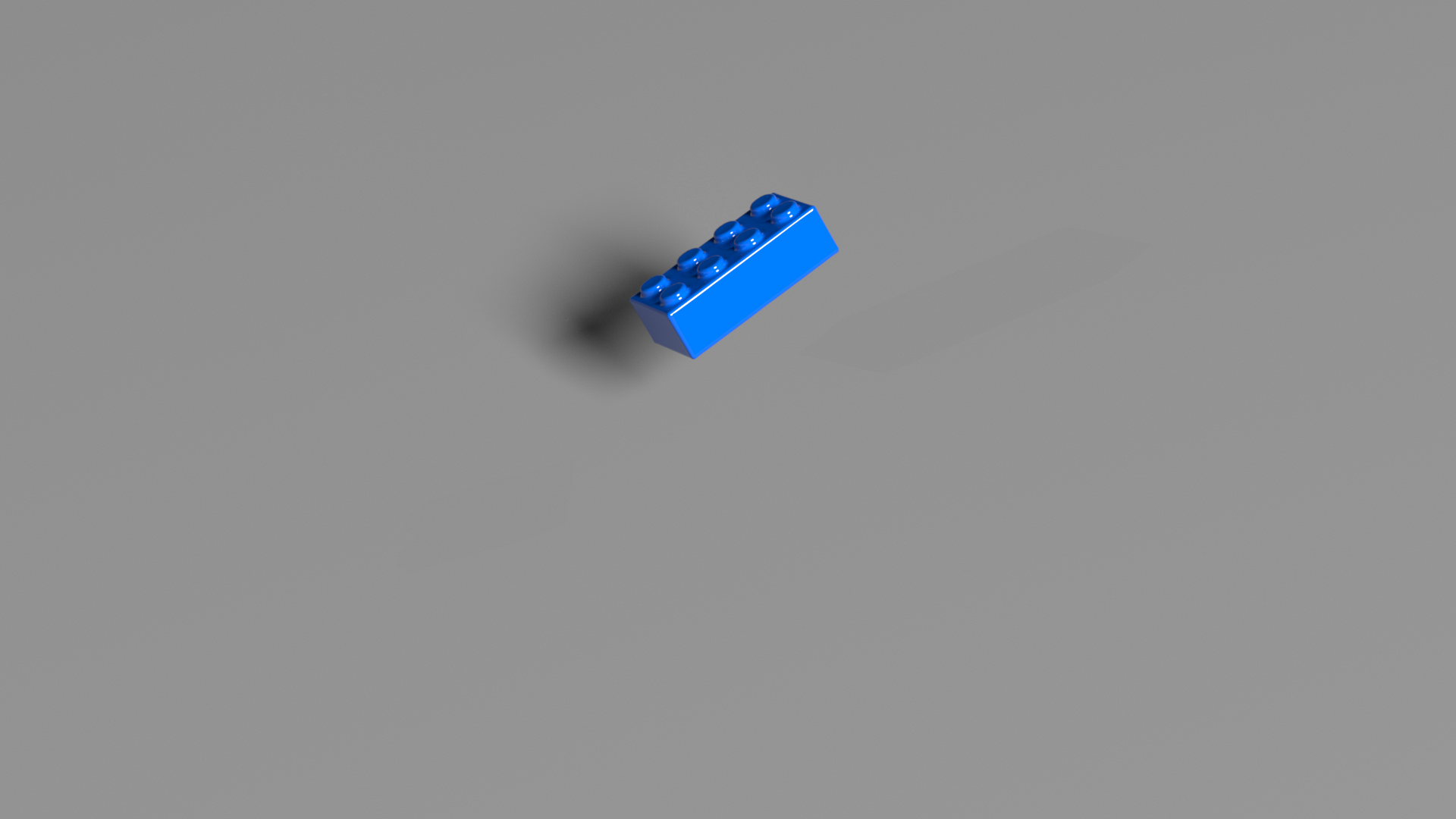
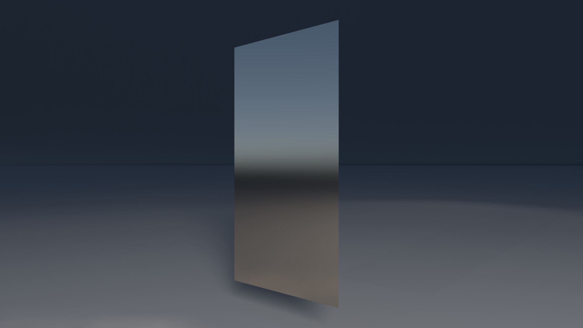
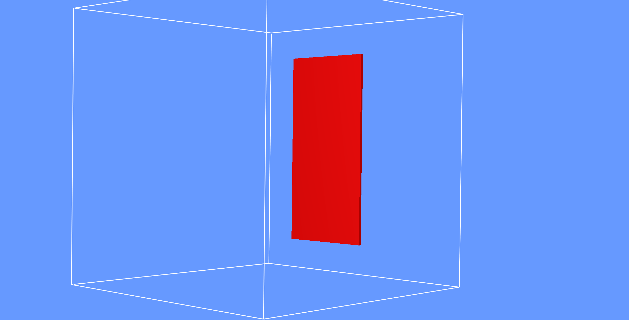
| LEGO (Rigid-bodies) |
 |
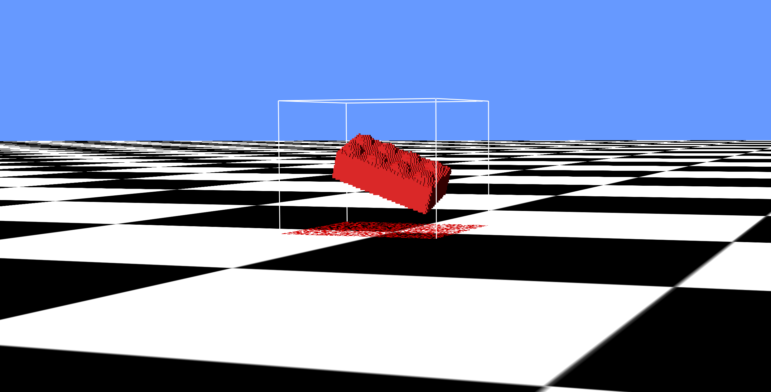 |
zip (149MB) | 1 | 50 | (0.008,0.015,-0.005) | 0.21 | 130k | 32 min | 320 | 2E-5 | (0.5,0.4,0.3) | 10 | 0.002 |
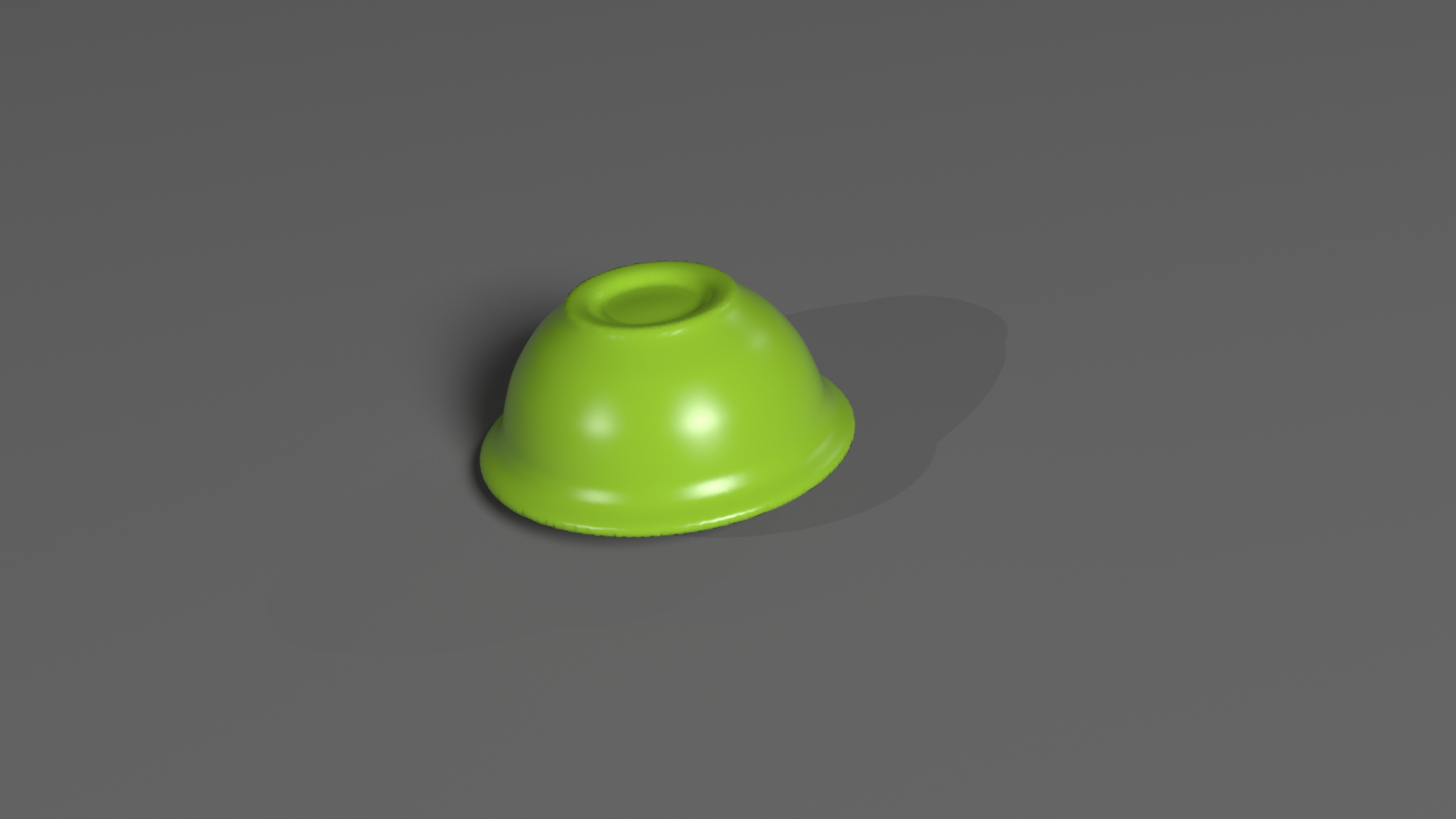
| Spolling Bowl (Rigid-bodies) |
 |
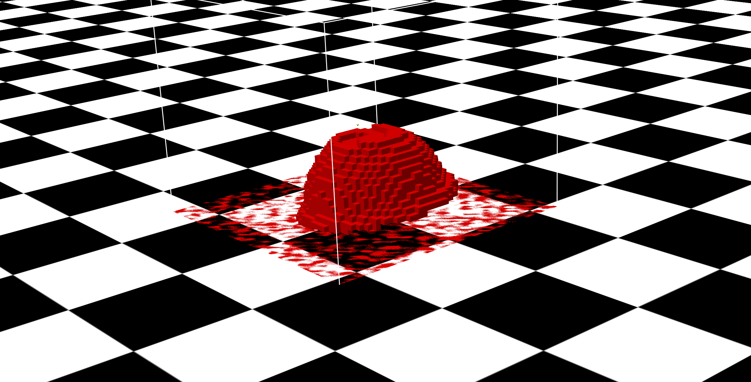 |
zip (152MB) | 5 | 50 | (0.0,0.08,0.015) | 2.5 | 300k | 63 min | 256 | 2E-5 | (0.5,0.4,0.3) | 8 | 0.1 |
| Wineglass Tap #5 (Rigid-bodies) |
 |
 |
zip (193MB) | 5 | 54 | (0.0,0.097,0.0) | 1 | 120k | 50 min | 36 | 2E-6 | (-0.5,0.4,-0.3) | 1 | N/A |
| Metal Sheet Shake (Thin-shells) |
 |
 |
zip (40GB) | 14.3 | 99 | (0.0,0.0,0.0) | 10 | 440k | 24 hr | 36 | 2E-6 | (3.0,0.0,4.0) | 1 | N/A |
| Cymbal (Thin-shells) |
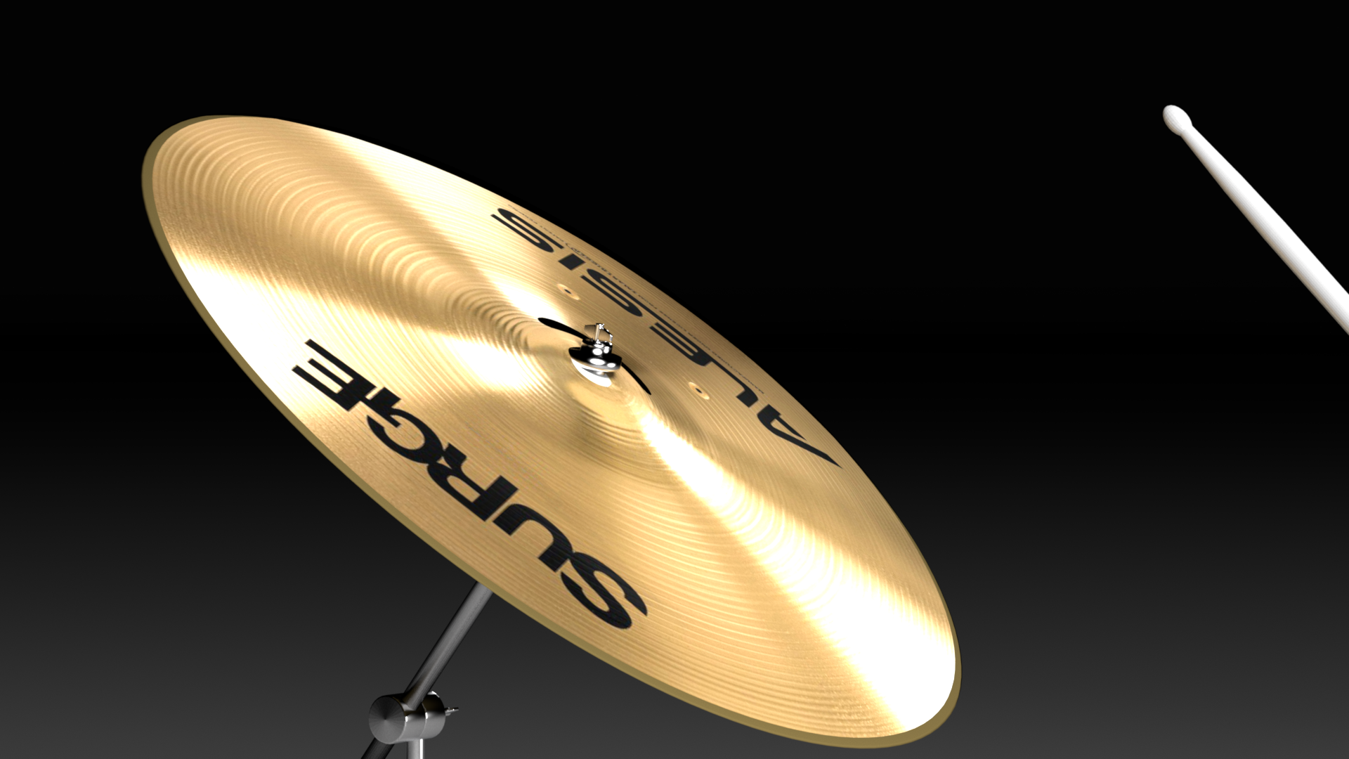 |
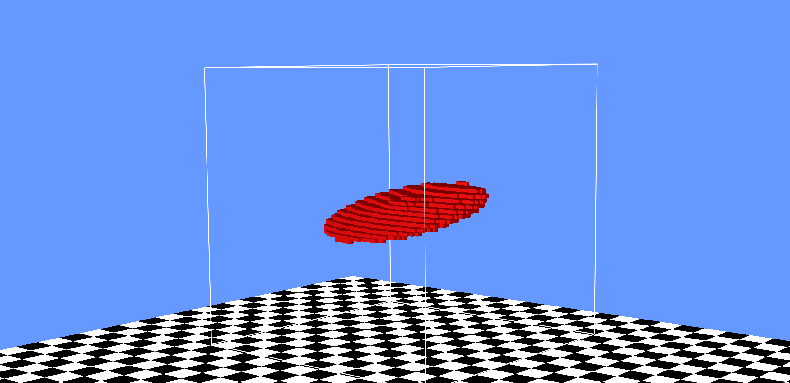 |
zip (9GB) | 10 | 80 | (-0.0003,0.716,-0.043) | 5 | 440k | 65 min | 640 | 2E-7 | (-1.879,0.716,0.684) | 1 | N/A |
| ABCD (Characters) |
 |
 |
zip (504MB) | 5 | 80 | (0.00,0.69,0.05) | 5 | 590k | 43-69 min | 256 | 2E-7 | (-0.001,0.686,0.5) | 8 | 0.5 |
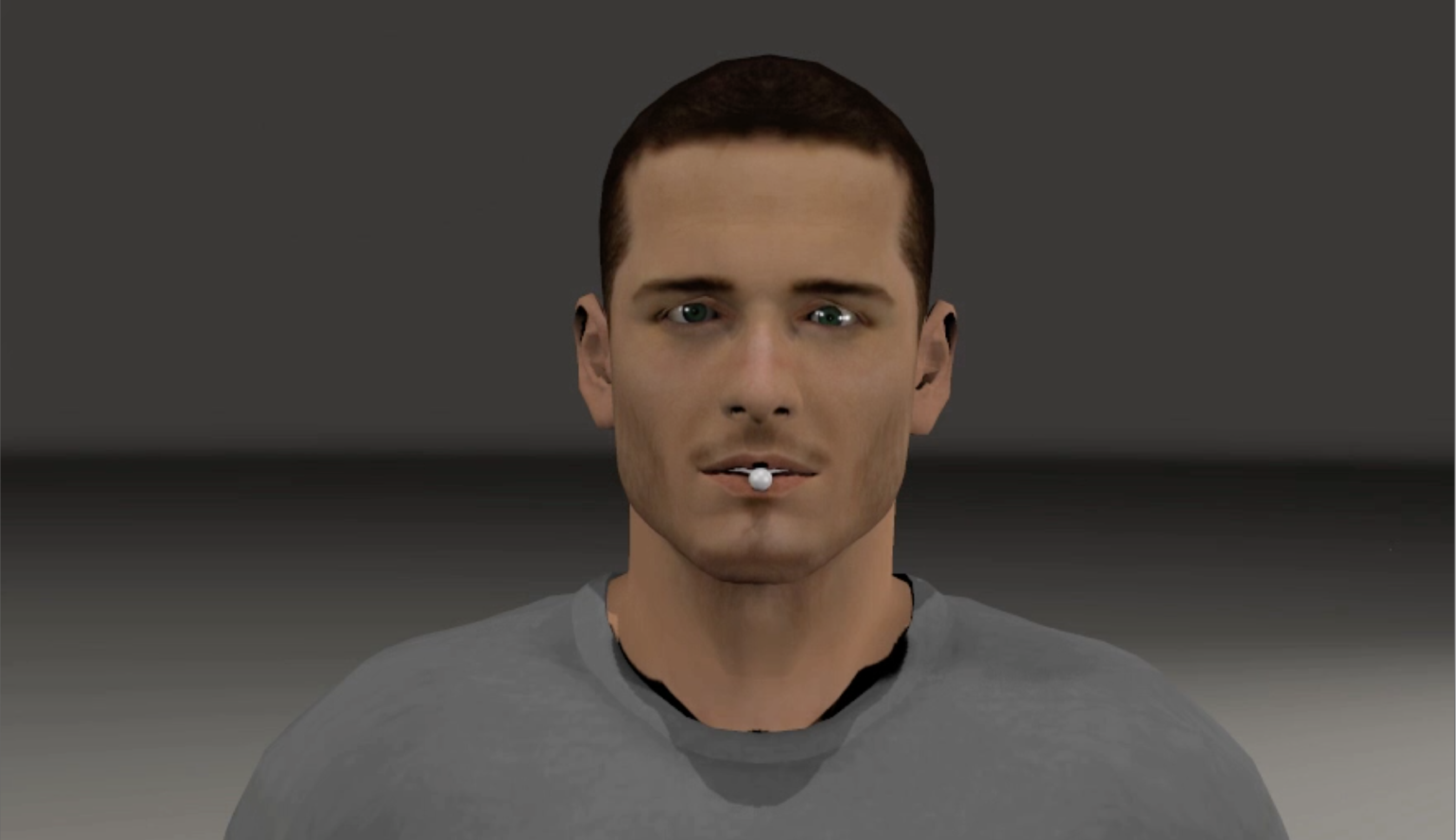
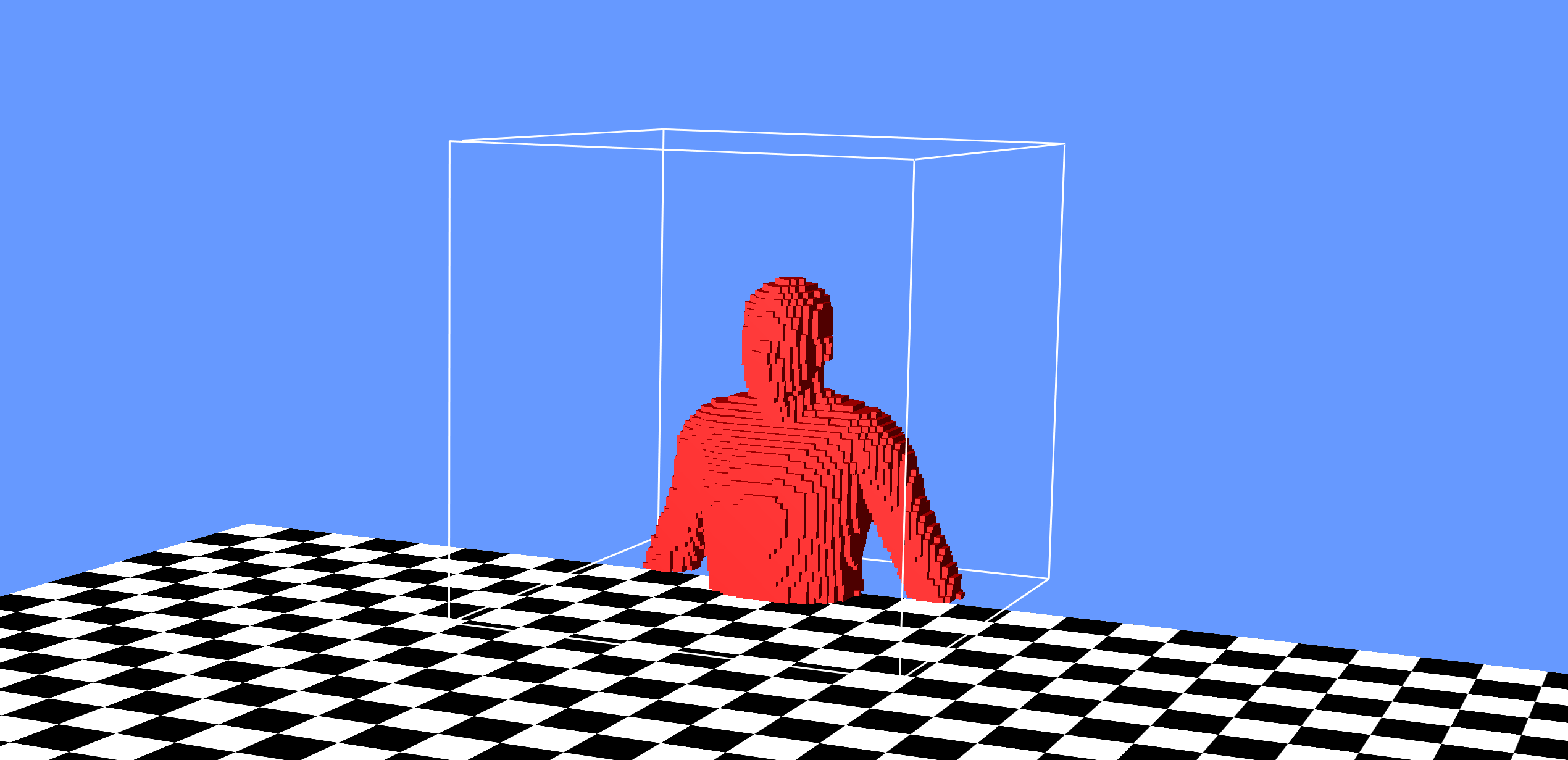
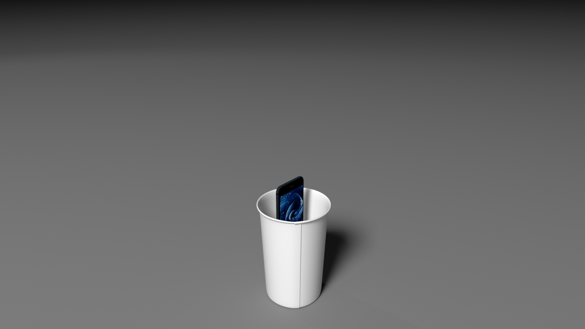
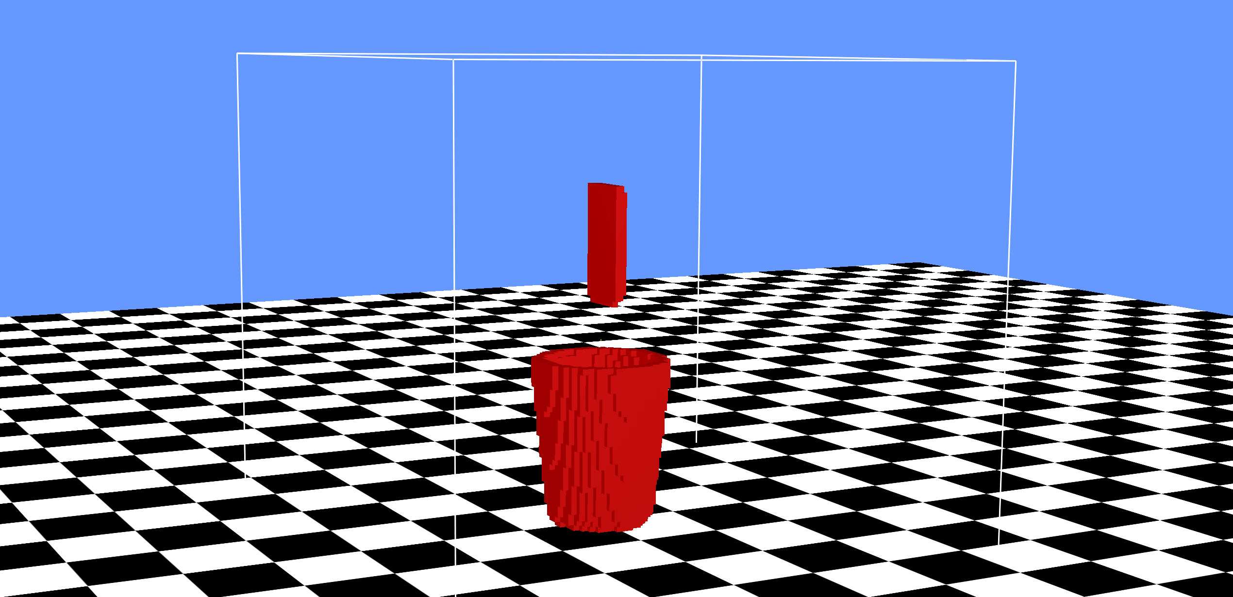
| Cup Phone (3D Re-recording) |
 |
 |
zip (5MB) | 7 | 90 | (0.0,0.217,0.0) | 8 | 710k | 41 min | 640 | 2E-6 | (0.43,0.54,0.53) | 20 | 0.0192 |
| Talk Fan (3D Re-recording) |
 |
 |
zip (9MB) | 10 | 85 | (0.0,0.97,0.0) | 10.5 | 930k | 67 min | 640 | 2E-7 | (0.06,0.948,1.26) | 20 | 0.025 |
| Trumpet (3D Re-recording) |
 |
 |
zip (3MB) | 10 | 70 | (0.01,0.20,0.05) | 11 | 970k | 33 min | 640 | 2E-5 | (-1.08,0.93,-0.574) | 20 | 0.05 |
h: cell sizes (mm)
L: grid dimension
C: grid center
T: time span for simulation
N: number of time steps taken
Runtime: wall-clock time for each run
N_t: number of cores (hyper-threaded) used for the runtime
measurement
alpha: viscosity coefficient
x_l: listening point
N_c: number of time-parallelization chunks
eps_i: maximum overlap time for time-parallelization chunks
Data Format
The zip file for each example contains the common file structure shown below. Most of the data files are stored in binary (little-endian). 8-byte doubles are used for floating point numbers unless specified otherwise. All binary files contain no line switch characters.
 ----- animation
   |
   --- misc
   |
   --- model
   |
   --- output
   |
   --- shader
animation contains representation of how the object is animated, such as transformations for rigid-bodies or keyframes for kinematic deformers.misc contains miscellaneous data, such as information for time-parallelization chunks.model contains object files used in the example, such as the Wavefront OBJ file.output contains output wav files at the listening positions.shader contains surface acceleration for each object.The above file structure description for each group of examples is described below.
Rigid-bodies
animation
displacement.bin is a binary file contains rigid-body transformations for each object. Translations and rotations are interleaved. The binary file format for a single timestep is explained below (d: double, i: integer). Our rigid-body solver is based on the impulsed-based method in [Guendelman et al. 2003].
d_time
i_id1   # first rigid object
d_translate.x d_translate.y d_translate.z
d_rot.w d_rot.x d_rot.y d_rot.z
i_id2   # second rigid obj
d_translate.x d_translate.y d_translate.z
d_rot.w d_rot.x d_rot.y d_rot.z
-1      # label the ending of this timestep
...
model
*.obj Wavefront OBJ files.
*.tet contains tetrahedral mesh corresponding to the obj file. The binary file format is explained below. Our solver is based on the isosurface stuffing algorithm [Labelle et al. 2007].
i_num_vertices # assume N+1
d_v0_x d_v0_y d_v0_z
d_v1_x d_v1_y d_v1_z
d_v2_x d_v2_y d_v2_z
...
d_vN_x d_vN_y d_vN_z
i_num_tetrahedrons # assume M+1
i_t0_i0 i_t0_i1 i_t0_i2 i_t0_i3
i_t1_i0 i_t1_i1 i_t1_i2 i_t1_i3
i_t2_i0 i_t2_i1 i_t2_i2 i_t2_i3
...
i_tM_i0 i_tM_i1 i_tM_i2 i_tM_i3
*.geo.txt Since in the wavesolver we only need the surface vibrational modes, a mapping is provided to cull all the volumetric modes. This file provides the mapping between the indices of the surface obj mesh, and the volumetirc tet mesh.
i_map_size
i_tet_index i_surf_index d_surf_normal_x d_surf_normal_y d_surf_normal_z d_area
i_tet_index i_surf_index d_surf_normal_x d_surf_normal_y d_surf_normal_z d_area
...
*.modes contains vibrational modes computed for the tetrahedral mesh. This file describes the modal frequencies (in terms of angular frequency squared) and modal matrix U in the rigid-body sound paper [Zheng et al. 2011]. The binary file format is explained below.
i_num_dofs # assume N+1
i_num_modes # assume M+1
d_omega_squared_0 d_omega_squared_1 ... d_omega_squared_M
d_u_0 d_u_1 ... d_u_N
shader
modalImpulses.txt contains impulses produced by our rigid-body solver. The text file format is explained below.
d_timestamp i_object_id i_vertex_id d_relative_speed d_impulse.x  d_impulse.y d_impulse.z c_T/S c_C/P
# C/P: constraint/pair impulse. T/S: S denotes the first and T the second object in the contact pair.
Thin-shells
Our solver is an extension of the unreduced FEM solver with an explicit leapfrog2 integration method introduced in [Chadwick et al. 2009], which is in turn based on the elastic thin-shell model in [Gingold et al. 2004]. The vertex displacement/acceleration data are computed and written to binary files, indexed by step indices at 44.1kHz. To satisfy the CFL condition, the integrator is running multiple substeps (for cymbal, 40 substeps) per outer step. To speed up the computation, we only recompute the damping matrix C every 16 outer steps. Internally, we reordered the vertex indices so that constrained vertices are stored at the end of the state vector (e.g. displacements, accelerations). That is, if a model has N vertices and n constrained vertices, then the displacement/acceleration vector is of size 3(N-n). The index map is provided in misc/vertex_map.txt. More details on the data format is described below.
animation
*.displacement contains displacement of the unconstrained vertices for a single timestep. The indices are the internal (reordered) indices. It is a binary vector, with format as follows:
i_num_dof # assume 3N+3
d_v0_x d_v0_y d_v0_z
d_v1_x d_v1_y d_v1_z
...
d_vN_x d_vN_y d_vN_z
*.constraint_displacement contains displacement of the constrained vertices for a single timestep. The format is the same binary vector file as *.displacement.
misc
vertex_map.txt contains the mapping between the original and the internal (reordered) vertex indices (0-based). The first column stores the original-to-internal map, and the second column stores the internal-to-original map. For example, consider the following vertex_map.txt
1 3
3 0
2 2
0 1
This mapping represents the following index pairs:
original internal
   0        1
   1        3
   2        2
   3        0
shader
*.wsacc contains acceleration of the unconstrained vertices for a single timestep. The indices are the internal (reordered) indices. It is a binary vector (see above for format).
*.constraint_acceleration contains acceleration of the constrained vertices for a single timestep. The indices are the internal (reordered) indices. It is a binary vector (see above for format).
Water
The folder structure for the water shader data is as follows:
shader
This folder holds meshes and bubble info. It contains the following folders:
bemOutput holds all the BEM solve data from [Langlois et al. 2016]. This is the surface acceleration data used in the wavesolver.
oscillators holds the tracking information of the bubbles.
The different files in these folders are described below:
bubbles-<time>.txt describes bubbles at the current time step. Format:
Bubble <id (1 based)> <radius> <avg pressure in bubble> <x> <y> <z>
deadBubbles-<time>.txt lists "dead" bubbles (have been alive long enough to finish ringing) at the current time step.
externalGmsh-<time>-<number of bubbles>.msh The surface that was used for external helmholtz solves.
fullOutput-<time>-<number of bubbles>.obj Entire simulation surface output in obj format.
gmsh-<time>-<number of bubbles>.msh
Entire simulation surface output in gmsh format. The different
types of surfaces are identified by their type. Fluid-air surface
triangles are type 1, rigid triangles are type 2, each bubble is
assigned a unique id starting at 3. Remember to subtract 2 from
this mesh bubble id to get to the 1 based indexing used elsewhere
(or subtract 3 to get to 0 based indexing used in a few places).
rigidBubbles-<time>-<number of bubbles>.txt
Lists "rigid" bubbles (bubbles that are touching the rigid
container walls).
info-<time>.txt
Stores the frequency of each bubble at this time step. The format is:
Time: <time>
<bubble id (0-based)> <frequency (Hz)> <pressure>
.
.
.
The frequency value is either a number, or DEAD (bubble stopped ringing, no velocity data available) or BAD (solve failed for some reason, no velocity data available).
helmSolution-<time>.dat
Stores the surface BEM velocity solution in binary. These files
match up to the externalGmsh files. The solution data is only
stored
for the fluid-air surface and the rigid surface. The data is stored
as std::complex<double>. At one time, for each bubble with a valid
frequency value in the corresponding info file, this files stores
the dirichlet ("pressure") data (one complex value for each
vertex),
and the neumann (velocity) data (one complex value for each fluid-
air triangle). The real part of each complex number is stored
first.
Little-endian format. The vertex/triangle ordering matches that in
the externalGmsh file.
trackedBubInfo.txt
Stores the bubble tracking information for the simulation.
For each entry in this file, the format is:
Bub <simulation-wide bubble id>
Start: <Type> <Time> <optional Bubble ids (simulation-wide)>
Radius <radius>
<Time> <Frequency> <Air Pressure> <Pressure in bubble> <Bubble id at simulation step (1-based)> <x> <y> <z>
.
.
.
End: <Type> <Time> <optional Bubble ids (simulation-wide)>
The start and end types can be:
N: new (entrained) bubble (only start type)
M: merged. The bubble ids that merged from or to are listed.
S: split. The bubble ids that split from or into are listed.
C: collapsed. Bubble collapsed (basically merged with the air).
3D Re-recording
For this class of examples, we generate a set of keyframes using animation software such as Blender. Each keyframe describes the transformation matrices and frame number. All objects are assumed to be rigid (no deformations allowed). At wavesolver runtime, the keyframes are interpolated (linear interpolation for translation and spherical interpolation for quaternion) to provide object positions to the solver. More details are provided below.
animation
*.kin contains kinematic descriptions of the keyframes. Specifically, frame index and the rigid transformations are provided. The text file format is described below.
i_frame d_translation_x d_translation_y d_translation_z d_quaternion_w d_quaternion_x d_quaternion_y d_quaternion_z
shader
input_wav/* contains the wav file we used for all the 3D re-recording shader (see paper for more details).
*_selected_vertices.txt contains an integer list of vertex indices (0-based) that we used to mask the area sound source. All vertices selected has acceleration corresponding to the input wav file, and all others have 0 acceleration.
Characters
Character examples have similar file/data structure to the 3D re-recording examples, except that now objects are allowed to deform. We first use the proprietary software Poser to generate character animations (with plausible lips motion), then we generate keyframes that contain wavefront OBJ files for each object. The geometries might not be topologically consistent (regarding the wavesolver), therefore the set of selected vertices are provided for each frame.