Assignment 3: Camera Simulation
Due: Friday May 5th, 11:59PM
Questions? Need help? Post them on the Assignment3Discussion page so everyone else can see!
Please add a link to your final writeup on Assignment3Submission.

Description
Many rendering systems approximate the light arriving on the film plane by assuming a pin-hole camera, which produces images where everything that is visible is sharp. In contrast, real cameras contain multi-lens assemblies with different imaging characteristics such as limited depth of field, field distortion, vignetting and spatially varying exposure. In this assignment, you'll extend pbrt with support for a more realistic camera model that accurately simulates these effects.
Specifically, we will provide you with data about real wide-angle, normal and telephoto lenses, each composed of multiple lens elements. You will build a camera plugin for pbrt that simulates the traversal of light through these lens assemblies. With this camera simulator, you'll explore the effects of focus, aperture and exposure. Using these data you can optimize the performance of your simulator considerably. Once you have a working camera simulator, you will add auto-focus capabilities to your camera.
Step 1: Background Reading
Please re-read the paper "A Realistic Camera Model for Computer Graphics" by Kolb, Mitchell, and Hanrahan.
Step 2: Implement a Compound Lens Simulator
Copy this zip file to a directory at the same as the directory containing the 'core' directory. This archive contains the following:
- A Makefile for Linux and a Visual Studio 2003 and 2005 project files for Windows.
- A stub C++ file, realistic.cpp, for the code you will write.
- Five pbrt scene files
Four lens description files (.dat files)
- Binaries for a reference implementation of realistic.cpp for Linux and Windows
Various textures used by the scene files located in the /textures subdirectory
Compilation Notes
If developing on Linux, the provided Makefile assumes you have placed your assignment 3 files in directory parallel to pbrt. (If you installed pbrt into ~/pbrt/pbrt/, then the Makefile assumes you've unzipped the assignment 3 files into ~/pbrt/YOUR_ASSGN_3_DIR/. If this is not the case, you'll need to change PBRT_BIN_DIR in the first line of the Makefile to point to your pbrt bin directory. Note that the Makefile is set up to copy the realistic camera shared object file to your pbrt bin directory for your convenience.
If developing on Windows, the provided project files assumes they are located in the pbrt/win32/Projects directory and that realistic.cpp is located in the /pbrt/cameras directory (You'll need to put it there). Visual studio 2003 and 2005 projects are provided and are located in the /vs2003 and /vs2005 subdirectories of the assignment 3 archive.
Binary reference implementations of a simulated camera are provided for Linux (realistic.so), Visual Studio 2003 (vs2003/realistic.dll), and Visual Studio 2005 (vs2005/realistic.dll).
Instructions
Modify the stub file, realistic.cpp, to trace rays from the film plane through the lens system supplied in the .dat files. The following is a suggested course of action, but feel free to proceed in the way that seems most logical to you:
Build an appropriate data structure to store the lens parameters supplied in the tab-delimited input .dat files. The format of the tables in these file is given in Figure 1 of the Kolb paper.
- Develop code to trace rays through this stack of lenses. Please use a full lens simulation rather than the thick lens approximation in the paper. It's easier (you don't have to calculate the thick lens parameters) and sufficiently efficient for this assignment.
Implement the RealisticCamera::GenerateRay function to trace randomly sampled rays through the lens system. For this part of the assignment, it will be easiest to just fire rays at the back element of the lens. Some of these rays will hit the aperture stop and terminate before they exit the front of the lens.
- Render images using commands such as 'pbrt hw3.dgauss.pbrt'. For your final renderings be sure to use the correct number of samples per pixel. The final handin should contain images rendered with both 4 and 512 samples per pixel.
You may compare your output against the reference implementation, (realistic.so on Linux and realistic.dll on Windows).
Here are some example images rendered with 512 samples per pixel: From left to right: telephoto, normal, wide angle and fisheye. Notice that the wide angle image is especially noisy -- why is that? Hint: look at the ray traces at the top of this web page.
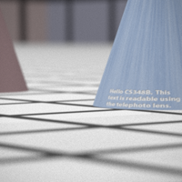
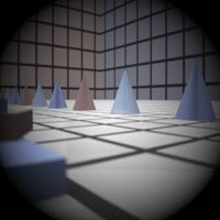
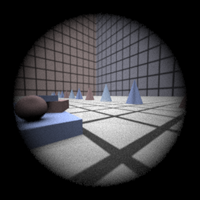
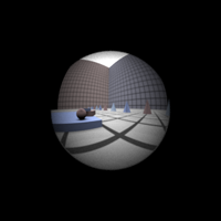
Some conventions:
- Assume that the origin of the camera system is at the left-most element of the stack (the point closest to the world).
Assume that the filmdistance parameter passed to the RealisticCamera constructor is measured from the right-most element of the stack (the point closest to the film).
There is exactly one aperture stop per lens data file. This is the entry with a radius of 0. Note that the diameter of this entry is the maximum aperture of the lens. The actual aperture diameter to use is passed in the scene file, and appears as a parameter to the RealisticCamera constructor.
- In this assignment, everything is measured in millimeters.
Hints:
ConcentricSampleDisk() is a useful function for converting two 1D uniform random samples into a uniform random sample on a disk. See p. 270 of the PBRT book.
- It may be helpful to decompose the lens stack into individual lens interfaces and the aperture stop. For the lens interfaces, you'll need to decide how to test whether rays intersect them, and how they refract according to the change of index of refraction on either side (review Snell's law).
- For rays that terminate at the aperture stop, return a ray with a weight of 0 -- pbrt tests for such a case and will terminate the ray.
Be careful to weight the rays appropriately (this is represented by the value returned from GenerateRay). You should derive the weight from the integral equation governing irradiance incident on the film plane (hint: in the simplest form, this equation contains a cosine term raised to the fourth power). The exact weight will depend on the sampling scheme that you use to estimate this integral. Make sure that your estimator is unbiased if you use importance sampling! The paper also contains details on this radiometric calculation.
- As is often the case in rendering, your code won't produce correct images until everything is working just right. Try to think of ways that you can modularize your work and test as much of it as possible incrementally as you go. Use assertions liberally to try to verify that your code is doing what you think it should at each step. Another wise course of action would be to produce a visualization of the rays refracting through your lens system as a debugging aid (compare to those at the top of this web page).
Step 3: Experiment with Exposure
Render a second image of the scene using the double gauss lens with the aperature radius reduced by one half. What effect to you expect to see? Does your camera simulation produce this result? When you half the aperture size, you have decreased the photograph exposure by how many stops?
Step 4: Autofocus
- You will now implement autofocus in your simulated camera. Digital cameras sample radiance within subregions of the sensor (film) plane called autofocus zones (AF zones) and analyze these small regions of the image to determine focus. For example, an autofocus algorithm might look for the present of high frequencies (sharp edges in the image) within an AF zone to signal the presence of an in focus image. You most likely have noticed the AF zones in the viewfinder of your own camera. As an example, the AF zones used by the autofocus system in the Nikon D200 are shown below.

In this part of the assignment, we will provide you a scene and a set of AF zones. You will need to use these zones to automatically determine the film depth for your camera so that the scene is in focus. Notice in the scene file autofocus_test.pbrt, the camera description contains an extra parameter af_zones. This parameter specifies the name of a text file that contains a list of AF zones. Each line in the file defines the bottom left and top right of a rectangular zone using 4 floating point numbers:
xleft xright ytop ybottom
These coordinates are relative to the top left corner of the film (the numbers will fall between 0.0 and 1.0). For example, a zone spanning the entire film plane would be given by 0.0 1.0 0.0 1.0. A zone spanning the top left quadrant of the film is 0.0 0.5 0.0 0.5.
You will need to implement the AutoFocus method of the RealisticCamera class. This method is called by the PBRT Scene class before rendering begins. In this method, the camera should modify it's film depth so that the scene is in focus.
There are many ways to go about implementing this part of the assignment. One approach is to shoot rays from within AF zones on the film plane out into the scene (essentially rendering a small part of the image), and then observe the radiance returned along each ray in an AF zone to determine if that part of the image is in focus. The zip file contains code intended to help you implement autofocus in this manner. Here are some tips to get started with the provided code:
The provided CameraSensor class is siimilar to the PBRT Film class but does not write data to files and can be cleared using the Reset() method. You can use this class to accumulate the radiance recieved within each AF Zone. the ComputeImageRGB() method will return a pointer to an array of floating point RGB values for your autofocusing logic processing.
SimpleStratifiedSampler is a modified version of PBRT's Stratified sampler plugin that is adapted for the needs of this project. The sampler to be reset and reused multiple times. You will need to pass samples generated by this sampler to the Scene::Li function.
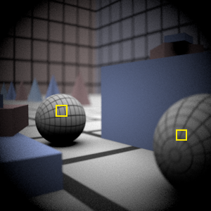
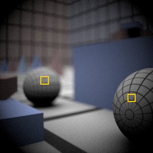
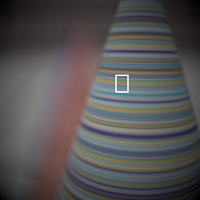
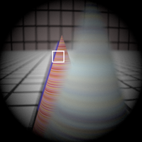
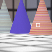
To test your autofocusing algorithm, we provide three scenes that require the camera to focus using a single AF Zone. The images resulting from proper focusing within the given AF zone hw3.afdgauss_closeup.pbrt, hw3.afdgauss_bg.pbrt, and hw3.aftelephoto.pbrt are shown below. We show the location of the AF zone in each image as a white rectangle.
More Hints
A heuristic for computing the sharpness of an image is the "Sum-Modified Laplacian" operator described in this paper by Sree Nayar.
- When generating subimages corresponding to the AF Zones, it will be important that you use enough samples per pixel to reduce noise that may make it difficult to determine the sharpness of the image. By experimentation, I've found that 256 total samples using the Sum-Modified Laplacian gives stable results.
- Although the autofocusing approach described here involves analyzing the image formed within each AF zone, an alternative approach would be to compute focus by using the depth information of camera ray intersections with scene geometry. Using the thick lens approximation from the Kolb paper, it should be possible to compute focus more efficiently than the approach described thus far.
Note that the CameraSensor contains (commented out) code to dump the current image to disk. This can be very useful in debugging.
Step 5: Submission
Create a wiki page named 'Assignment3' under your home directory that includes a description of your techniques and your final rendered images, and post a link to this page on Assignment3Submission. Please be sure to render images using the required number of samples per pixel and describe in detail how you implemented your autofocus algorithm in the writeup. In your writeup, please follow the layout of the page template given Assignment3Template. Your grade in this assignment will be determined by the quality of your rendered images, the ability of your autofocus algorithm to produce in-focus images on the provided sample scenes, and on your writeup. Extra credit will be given for cleverness in your autofocusing implementation. As in the previous assignment, please do not include your source file in the wiki page. Send an email to cs348b-spr0506-staff@lists.stanford.edu with subject "cs348b HW3" and your realistic.cpp as an attachment.
Optional Extras
To investigate cameras further, we encourage you to try the following (the following are NOT required parts of the handin for assignment 3):
Stop Down the Telephoto Lens
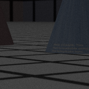
In the telephoto lens scene (hw3.telephoto.250mm.pbrt), change the aperture so that the exposure is decreased by 4 stops. If you have photoshop, you can check to see if your simulation is correct by increasing the brightness of the resulting EXR file by 4 stops (increase exposure by 4 on the exposure slider). Other than the change in exposure, what else changes in the resulting image when you stop down the lens? Here is a reference image:
More Complex Auto Focus
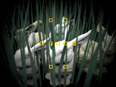
Here are some more complex scenes to try your autofocusing camera on. The scene data files are provided here, just place them in the same directory as your other assignment3 scenes. The scene containing the bunnies references geometry stored in /afs/ir/class/cs348b/assignments/geometry, so you might have to change paths accordingly. These scenes comes with autofocus zone files containing multiple zones. Like any any digital camera, what zone you choose to select focus from determines whether your autofocus will converge on a foreground or background object. It would be interesting to see how your algorithm fares on these scenes. Perhaps you might want to add a parameter to the scene file (see CreateCamera at the bottom of realistic.cpp to see how) to tell you camera to prioritize foreground or background objects (just like switching on "macro-mode" is a hint to your digital camera). The following images are rendered at 128 samples per pixel, AF zones are shown on the images.
