Assignment 3 Camera Simulation
Joyce Pan
Date submitted: 08 May 2006
Code emailed:08 May 2006
Compound Lens Simulator
Description of implementation approach and comments
I read in the lens parameters similarly to the autofocus parameters, creating a struct of all the values we needed to keep track of and putting them in a vector. Then I translated the sample point into a point on the film plane using the film diagonal as a reference. I fired the ray at the back lens using ConcentricSampleDisk(). Then for each lens in the camera (except the aperture), I'd intersect the ray with the sphere created by the edge of the sphere and pick the edge on the side that the lens was on. Since we already know the point is on the sphere, to see if it's on the lens, I simple looked at it's distance from the origin in the xy plane to see if it was less than the lens radius. The normal was calculated as the intersection - the center of the sphere. If the radius was negative, the normal ray was reversed. I calculated Snell's law using the wikipedia equation. If either the ray didn't intersect the sphere within the lens or the equation for Snell's law created a negative square root, then the ray was rejected.
The weight was calculated with A/(Z2)*cos4, where the A and Z were derived with respect to the back lens, meaning Z was filmdistance and A was just the area of the back lens, no testing necessary based on refracting light rays. After weighting the ray, I readjusted it so that its origin was on the near plane, set tmin to 0 and adjusted tmax to the far plane.
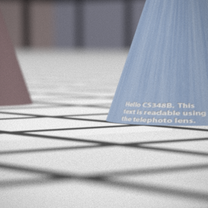
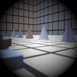
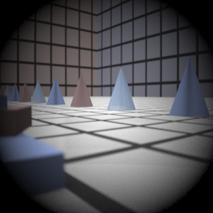
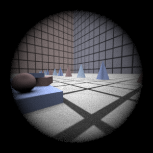
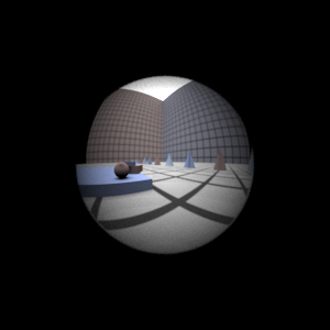
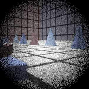
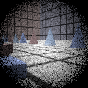
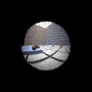
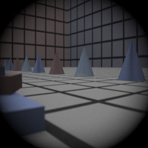
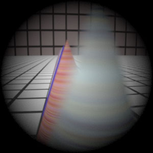
Final Images Rendered with 512 samples per pixel
|
My Implementation |
Reference |
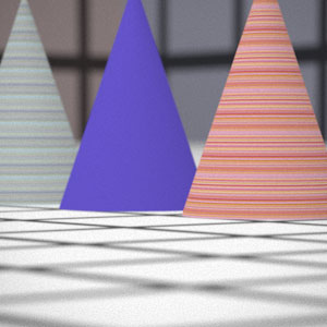
Telephoto |
|
|
Double Gausss |
|
|
Wide Angle |
|
|
Fisheye |
|
|
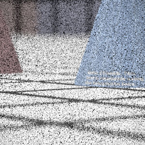
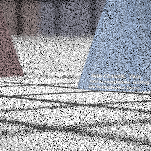
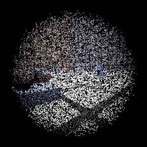
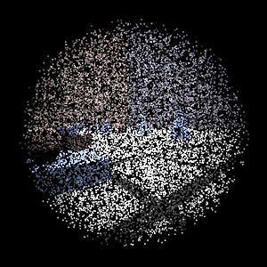
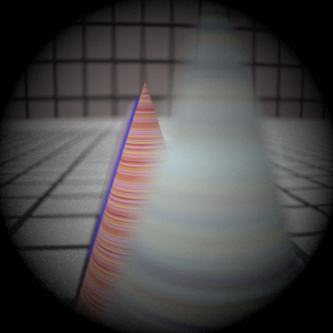
Final Images Rendered with 4 samples per pixel
|
My Implementation |
Reference |
Telephoto |
|
|
Double Gausss |
|
|
Wide Angle |
|
|
Fisheye |
|
|
Experiment with Exposure
Image with aperture full open |
Image with half radius aperture |
|
|
Observation and Explanation
Halving the radius is the equivalent of stopping the exposure down 2 stops. As a result, many more rays get rejected and the image is 1/4 the brightness.
Autofocus Simulation
I used the SML equation given in the paper, using (r+g+b)/3 for the image intensity. Then I calculated the standard deviation of the SML for the sample. Since the pattern seemed to be very high standard deviations towards the back lens, decreasing as we got farther, I started sampling at the back with a 2.5 step size so as not to miss very sharp and narrow peaks.
It was hard to decide what criteria to look for. After looking at the data values I got, I decided to look at all the peaks, keeping a running track of local max and mins. I also kept track of the average standard deviation so far. If the distance between the max and min on both sides of a peak was more than twice the average standard deviation, this was decided to be a peak, and the search terminated.
Since 2.5 is a somewhat large step, I then looked at the values that were 2.5 less than the film distance to 2.5 above the film distance, taking steps of 0.5. This time, instead of looking for peaks, since we already know this is a peak, I took the highest value.
It turns out that 2.5 is a pretty decent step, but I think it's partially because the values tended towards multiples of 2.5 If it were straddling in the middle, then the extra 0.5 step would be helpful.
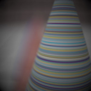
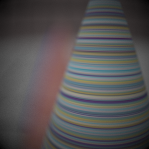
Final Images Rendered with 512 samples per pixel
|
Adjusted film distance |
My Implementation |
Reference |
Double Gausss 1 |
61.5 mm |
|
|
Double Gausss 2 |
37.5 mm |
|
|
Telephoto |
117.5 mm |
|
|
Any Extras
|| ||
||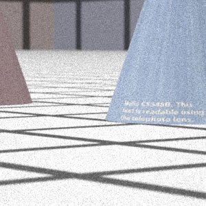 ||
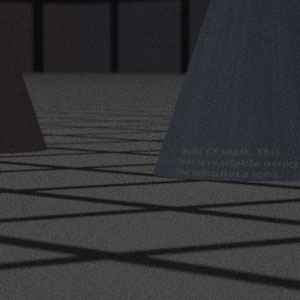
|| To stop down the telephoto lens by four stops, I divided the aperture radius by 4. Although increasing the exposure in Photoshop restores the brightness and contrast, the image is grainier, since less rays make it through the aperture, so the sampling decreases significantly.
