• RanjithaKumar
• FinalProject

You are not allowed to do AttachFile on this page. Login and try again.

Final Project: Rendering Lily Pads

Tom Brow, Ranjitha Kumar

Introduction

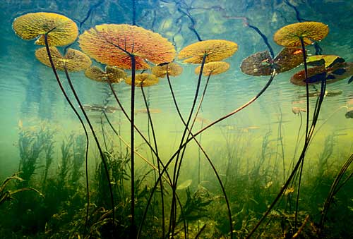
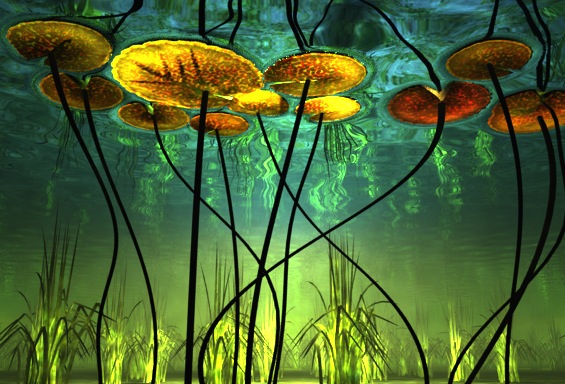
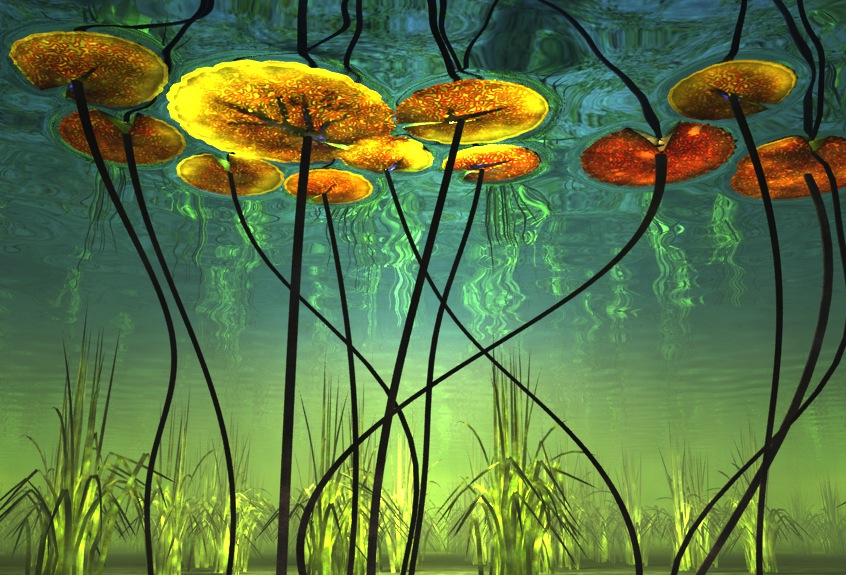
We wanted to reproduce an underwater photograph of lilypads by photographer Frans Lanting. Our solution involves procedural modeling, subsurface scattering, and multiple volume scattering.

Lily Pad Models (Ranjitha)

All the lily pads and stems were modelled in Mathematica; the screen shot below shows the basic form of the equations used to model both the pads and the stems. The intuition used to create the lily pad models is as follows:

• {x(u,v) = cos(u), y(u,v) = sin(u), z(u,v) = C} creates a circle in the z(u, v) = C plane.
• To create a circle with frills on the outer edge, add cosine terms of varying frequency and amplitude to x(u, v) and sine terms of varying frequency and amplitude to y(u, v).
• Varying u from 0 to a value less than 2*Pi, results in an incomplete circle. To make the circle pucker inwards like a cardiod, multiply x(u,v) and y(u,v) by some degree of v.
• The other terms in x(u,v) and y(u,v) are used to move the location of the center of the lilypad so that stem is not attached to the dead center of the circle.
• Finally, defining z(u,v) as sin(v) makes the lily pad curve inward to meet the stem.

The model of the lily pad stems can be thought of as sweeping a circle along a curve defined by sines and cosines.

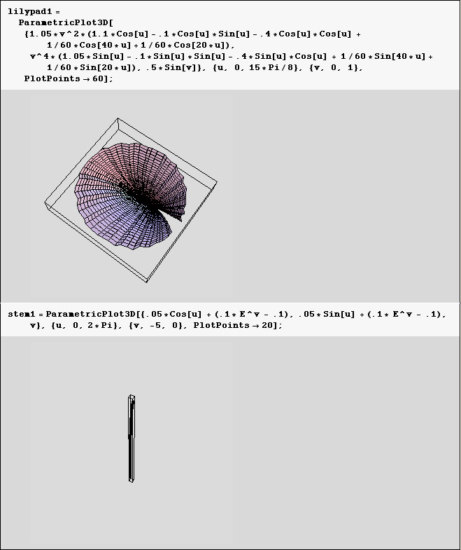
After creating all of the models in Mathematica, the geometry was outputted to PBRT scene files and referenced in the main scene file. We used the Mathematica to PBRT converter available at http://pbrt.org/downloads.php. Rotations and translations were applied to the models to place them so they closely matched up with the original photo.

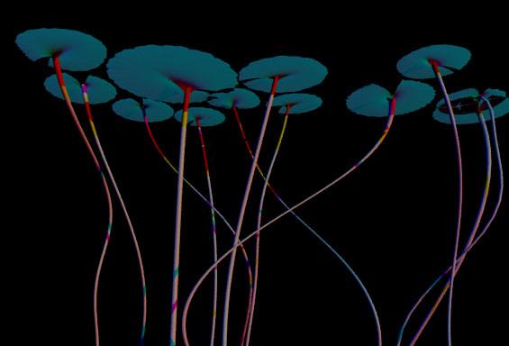
Subsurface Scattering (Ranjitha)

Since the lily pads are so thin, we modeled single-layer, single-scattering subsurface scattering. In PBRT, we defined a new type of material for the lily pad. It consists of a rough specular BRDF with a specular exponent of 10 [1], a subsurface scattering BRDF, modeling backscattering from a single-scattering event, and a BTDF, modeling the attenuation due to transmission through a homogeneous volume.

The rough specular BRDF is important to capture the waxy highlights of lilypad surface [1], and the subsurface backscattering and transmission are important to capture the translucency and the color bleeding effects.

The reflection.cpp file is augmented to include functions for the 1st-order (single-scatter) BRDF and 0th-order (no scattering) BTDF. (Uniform hemisphere sampling is used for sampling the BRDF and BTDF.)

The backscattering integral for the single-scattering model has a closed form: W*(T12)*(T21)*p(omega_i, omega_r)*(cos(theta_i))/(cos(theta_i)+cos(theta_r))*(1-e^{(-tau_d(1/cos(theta_i)+1/cos(theta_r)))}), where W represents the albedo, T12 and T21 are the Fresnel boundary terms, and p is the phase function, and tau_d is the optical depth, equivalent to sigma_t*depth [1]. The (1-e^{(-tau_d(1/cos(theta_i)+1/cos(theta_r)))}) term reflects the boundary condition from 0 to a particular depth.

Here are some of the details involved in evaluating the terms in the closed form:

• Since plants are mostly made out of water, we initialize the lily pad to be a Fresnel dielectric with the index of refraction equal to 1.33 inside of the material [1].
• We compute the angles theta_i and theta_r by first refracting the incident and outgoing directions.
• For the phase function, we Henyey-Greenstein function with g = .3, which indicates mostly forward scattering [1].
• To compute the optical depth, we uniformly choose a depth between 0 and maximum thickness at the intersection point; this is where the scattering event occurs.
• The sig_t = sig_s + sig_a and albedo = sig_s/sig_t are both passed in as parameters. We assume uniform sig_t along the depth, therefore, the optical depth is equal to the product of sig_t evaluated at the intersection point and depth at which the scattering event occurs. We also define sig_t and W to be Spectrum objects because we would like to determine which wavelengths of light are more absorbed than others (sig_a), and which ones are more scattered than others (sig_s) at a given intersection point.

The 0th-order BTDF for subsurface scattering is nothing but the attenuation due to a ray traveling through a homogeneous medium: (T12)*(T23)*e^(-tau_d), where T12 and T23 are the Fresnel boundary terms, and tau_d is the optical depth [1]. The optical depth is evaluated to be the product of sig_t (which is again assumed to be uniform along the depth) and the thickenss at an intersection point.

From the scene file we obtain values for sig_a and sig_s which are then used to calculate the albedo and sig_t which are passed into the constructors of the subsurface BRDF and BTDF in lily pad material. To make it easier to control the parameters we keep sig_s constant throughout the material and vary sig_a using a texture map. Texture maps are also used to modulate depth and Ks, the color of the rough specular term.

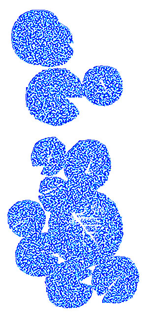
Below is a rendering of the lily pads showcasing the final lily pad material with all the texture maps used.

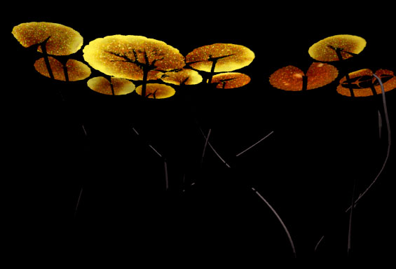
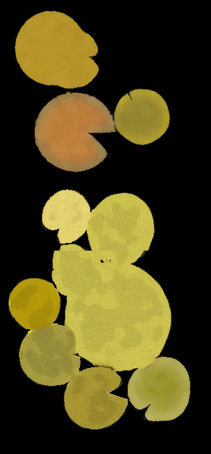
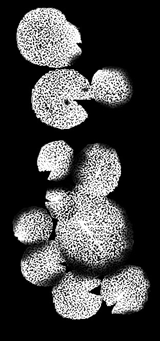
These are all the texture maps that were created and mapped onto the lily pads. Notice how the brown and red shades come from the sig_a and depth texture maps. The ks texture map mostly assigns shades of green to all the lily pads. We noticed that there had to be a correlation between the sig_a and the depth maps to really get the dark red bumps on the lily pads. If we had more time, we would have liked to procedurally generate vein textures for a more realistic appearance.

Multiple Volume Scattering (Tom)

Because the only light entering the visible part of our scene comes through the surface of the water, all of the light that reaches the eye is multiply scattered. So although our scene doesn't exhibit the volume caustics or "god rays" that usually motivate volumetric photon mapping, we needed to implement it anyway.

Following [2] and [3], we extended pbrt's built in photon mapping surface integrator, photonmap, to store a volume photon map as described in [4]. Whereas the original photonmap shoots a ray from the light source and stores a photon at every point the bouncing ray hits a surface, our extended version allows the ray to be scattered or absorbed at any point in the volume, and stores photons for those interactions as well. The result is a collection of photons that can be used by a volume integrator to estimate the in-scattered radiance at any point.

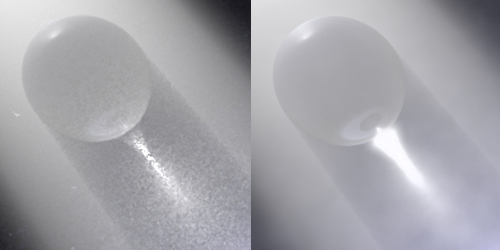
[4] does not specify a method for determining whether and where a volume interaction occurs. Given a ray through a volume, [2] considers the 1D cross section along the entire length of the ray and samples a t value accordingly. [3] marches along the ray from mint to maxt by randomly-sized intervals, using the transmittance over each interval to determine the probability that an interaction occurs there. If there is an interaction, the upper bound of the interval is the t where it occurs. Because of this rounding up, method [3] is biased towards a higher value of t, which results in incorrect-looking volume caustics unless the size of the intervals is small. Since the cost of ray marching is inversely proportional to the interval size, we decided to remove the bias.

Our method combines the two methods described above. Like [3], we step along the ray by intervals, using the interval transmittance to test for an interaction. But if an interaction does occur, we randomly sample a point within the interval for the location of the interaction. We assume that transmittance is uniform within the interval, such that we can analytically calculate the PDF from which we need to sample to correctly select the location. The volume caustics generated by this method appear correct in homogeneous volumes even with large interval sizes.

Another challenge we ran up against was "blotchiness" -- bright, jarring spheres of light around very high-weighted photons. Fortunately for us, this problem occurs in surface photon mapping as well, and has been addressed in the extended photon mapping surface integrator, exphotonmap (available here). One strategy the new integrator implements is an improved form of russian roulette ray termination during photon shooting; higher-weighted rays are less likely to be terminated, and thus have their weight divided by a greater amount if they are not terminated. The result is a more uniform distribution of weights over photons in the map, eliminating blotches. It was easy to adapt this improvement into our own volumetric photon mapping code.

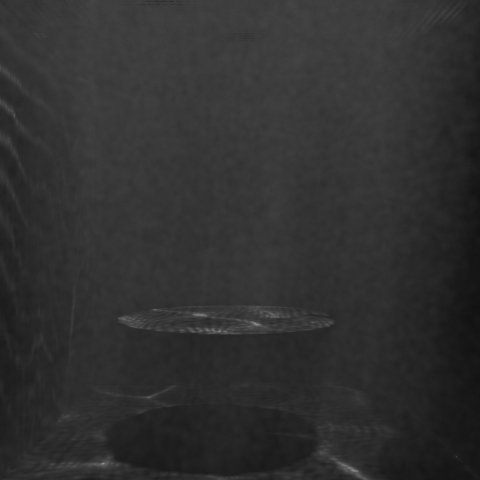
Finally, we modified the single volume integrator to include the in-scattered indirect light as given by the volume photon map. The integrator's original code is used to handle direct light.

Surface Interactions (Tom)

Lily pads straddle the border between water and air, with their top sides above the surface and their bottom sides below. To make it easy to align the lily pads in this way, we modeled the surface as a bump-mapped plane rather than a heightfield. The topmost part of the lily pad (the edge) is an imperceptibly small distance below the plane.

This configuration alone didn't accurately model the scene because incoming light still interacted with the water surface above the lily pad. The pads were visibly darker as much of the light was reflected back off the water. To account for the fact that the tops of the pads are above water, we defined the index of refraction above the pads to be 1. We specified index of refraction using a planar-mapped texture, which itself was simply an orthographic projection of the lily pads onto the plane of the water surface.

We were also able to use this texture to create the illusion of surface tension. We blurred the texture slightly and applied it as a bump map, such that the normal of the water surface was perturbed around the edges of the lily pads. To incorporate waves, we interpolated between this surface tension texture and pbrt's provided fbm "turbulence" texture for our final bump map.

References

[1] Hanrahan, Pat and Wolfgang Kreuger. "Reflection from Layered Surfaces due to Subsurface Scattering". Proc. SIGGRAPH, 1993.

[2] Fatahlian, Kayvon and Tim Foley. "Rendering Jellyfish".

[3] Hong, Chris and Garrett Smith. "Rendering Underwater Scenes".

[4] Jensen, Henrik Wann and Per H. Christensen. "Efficient Simulation of Light Transport in Scenes with Participating Media using Photon Maps". Proc. SIGGRAPH, 1998.