Assignment 3 Camera Simulation
Sean Rosenbaum
Date submitted: ?? May 2006
Code emailed: ?? May 2006
More images on the way!!!!
Compound Lens Simulator
Description of implementation approach and comments
FILL ME IN!!!!!!!!!!!!!!!!!!!!!!!!!!!!!!!!!!!!!!!!!!!!!!!!!!!!!!!!!!!!!!!!!!!!!!!!!!!!!!
Debugging
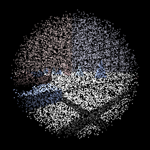
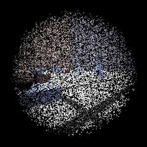
Once all the code for tracing rays through the lens was in place, I found my implementation too bugged to produce meaningful results. While I managed to track down several bugs using the debugger, I was still getting junk. I verified my transformations were working correctly by substituting pbrt's perspective camera into my code. This confirmed that my tracing was to blame. After several hours of frustation, I decided to produce a visualization as suggested in the assignment description. The visualization shows where each lens is located, the path of rays through the system, the normals of the elements they hit, and their refraction direction. For simplicity, the visualization is in 2D, with the top display showing the lens from the (-z)-x plane and the bottom the (-z)-y plane. This visualization helped immensely. Shortly after it was in operation I managed to hunt down the remaining bugs.
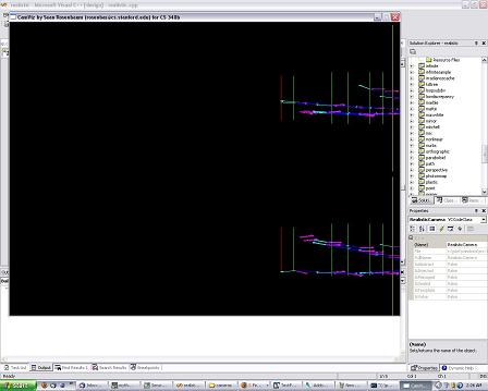
Here each interface comes into view once a ray tests for intersection against it. Only a single vertical line is drawn for each interface, which is located where the elements has the disk of max aperture. The intersection normal and refraction direction emanate from the actual points on the surfaces they intersect. The entire process is animated so that it's easy to follow along one step at a time.
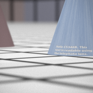
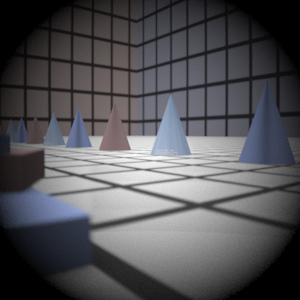
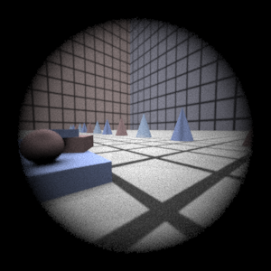
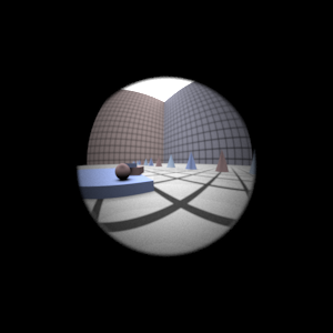
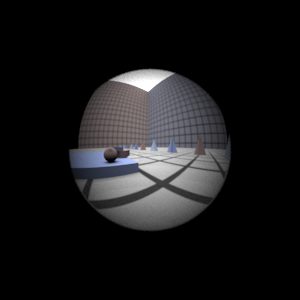
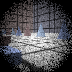
Final Images Rendered with 512 samples per pixel
|
My Implementation |
Reference |
Telephoto |
|
|
Double Gausss |
|
|
Wide Angle |
|
|
Fisheye |
|
|
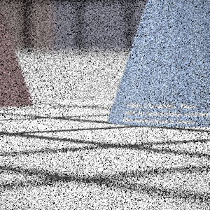
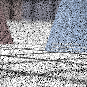
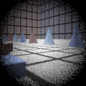
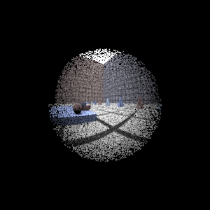
Final Images Rendered with 4 samples per pixel
|
My Implementation |
Reference |
Telephoto |
|
|
Double Gausss |
|
|
Wide Angle |
|
|
Fisheye |
|
|
Experiment with Exposure
Image with aperture full open |
Image with half radius aperture |
|
|
Observation and Explanation
FILL ME IN!!!!!!!!!!!!!!!!!!!!!!!!!!!!!!!!!!!!!!!!!!!!!!!!!!!!!!!!!!!!!!!!!!!!!!!!!!!!!!
Autofocus Simulation
Description of implementation approach and comments
My algorithm relies heavily on the Sum-Modified-Laplacian (SML) to approximate the focus for a several film distances. The SML is computed for the autofocus zone at a given film distance using the intensity of the RGB values (i.e. max(R,G,B)) given by the camera sensor. In order to find the optimal film distance, I treated this as a one-dimensional optimization problem over a unimodal function. To keep my autofocus flexible, I set my search range to be very large, ranging from 0 to 220mm regardless of the camera used. Obviously effectively searching over a range like this large requires a fast and robust search. I first attempted to do a bisection-like search over the search range. This entailed taking two sample film distances near the center of the interval, computing the SML for each, and then continuing on to the interval on the side of the sample with the greater focus. Technically, the subinterval between the two samples is also included, as the maximum may fall within it. After this was fully functional, I was disappointed in how slow it went because the focus calculations are quite expensive, specifically because I ramped up the number of samples to virtually eliminate noise. After perusing some literature on 1D optimization, I found that I could get by doing only one SML for each iteration, rather than two, by doing a golden section search. This algorithm is similar to the previous one. The general idea is to pick a sample position in the interval that can be reused in subsequent iterations. However, it is subject to the constraint that during each iteration, the current pair of points have the same relative positions in their interval as the previous points had. This ensures we continue to shrink the interval by a constant fraction at each iteration. This cut the autofocus time roughly in half.
Unfortunately, I ran into trouble doing these types of searches. The main problem was the SML was subject to error given that it is only an approximation. Consequently, my search would sometimes skip over a subinterval containing the optimal distance. My solution was to subdivide the search-range into several intervals, run the golden-section search on each one, and take the best film distance. The intervals vary in size. They gradually get larger as the distance from the back lens increases. This technique made my autofocus much more robust, though a bit slower. It can be made nearly as fast as a single golden-section search by immediately halting the computation for some of the intervals once it's apparent the optimal distance lies outside it. For instance, if a reasonably good focus is found in one interval, there's probably no need to search other far off intervals. Also, if the focus seems extremely bad when an interval is started, there's probably no need to continue searching it. I took advantage of this by immediately halting computation for any intervals encountering several consecutive SML results below some fraction of the current best from prior intervals, or below a predefined threshold. This halting behavior makes the algorithm even more effective at searching large intervals. The search range can be made much larger without a significant impact on performance, though I didn't see the point of making it even larger since none of these images even got remotely close to the far end of it.
I handle several autofocus(AF) zones by replacing the SML above with a sum of SMLs, each term weighted by the area of its zone. This simply attempts to optimize the focus over all the zones. The bunny scene at the bottom of the page demonstrates that in practice this does quite well.
Future Work
Successive parabolic interpolation may be more efficient than golden-section search given it's faster convergence rate. This technique works by sampling several distances, forming a parabola over the results, computing the minimum of this parabola, and successively refining it.
SML has several parameters, including a step size for computing MLs and a minimum threshold for summing them. I set these as one and zero, respectively. I suppose tweaking them some more may lead to even better results.
Like I said before, I used a lot of samples for rendering the AF zones to get rid of noise across the entire search range. This is one reason why my images are in such great focus despite the large search range. A potentially better approach would be to render them with fewer samples and then do some image processing on the noisy ones. Doing so may give a huge boost to performance, while not significantly impacting the autofocus quality.
References
Shree K. Nayar. Shape From Focus System. IEEE Conference on Computer Vision and Pattern Recognition (CVPR), pp.302-308, Jun, 1992.
Michael T. Heath. Scientific Computing, An Introductory Survey - 2nd Ed. McGraw-Hill, 2002.
Final Images Rendered with 512 samples per pixel
|
Adjusted film distance |
My Implementation |
Reference |
Double Gausss 1 |
62.1 mm |
|
|
Double Gausss 2 |
39.8 mm |
|
|
Telephoto |
117.1 mm |
|
|
Any Extras
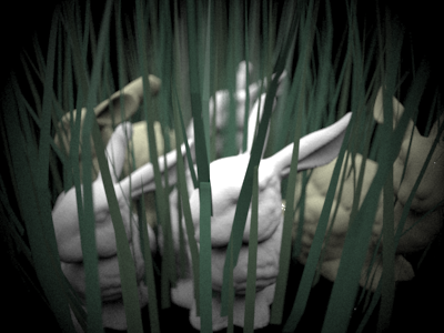
Autofocus with multiple AF zones. Film distance of 39.9mm
