Assignment 3 Camera Simulation
Shradha Budhiraja
Date submitted: 05 May 2006
Code emailed: 07 May 2006
Compound Lens Simulator
Description of implementation approach and comments
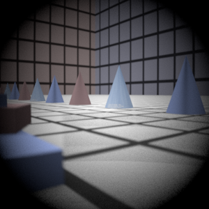
The lens simulator works on the basic principles of refraction through glass. At first, it was important to convert the raw image coordinates given by the sample to appropriate camera coordinates. This was done by computing the screen extent using the film diagonal and the horizontal and vertical resolutions and transforming the raster coordinates using this. This became the origin of the ray. Samples on the lens were taken on the back surface of the last lens in stack. Also, the position of the camera is in the negative z direction at a distance of filmdustance plus the thickness of the entire lens system. Thus these two points on the lens and the film determined the original direction of the ray. This was normalized and thus used to calculate cos(theta) , where theta is the angle the initial ray makes with the normal of the image plane, for the weight term. The total weight of the ray was given by the product of the area of the disk and the fourth power of cos(theta) all divided by the square of the film distance.
The next step was to perform the sphere-ray intersections as the ray passes through each lens in stack. This was done by simply plugging the equation of a ray (o + td) into the equation of a sphere and solving the quadratic in t. If the intersection point is beyond the aperture, the ray does not make it to the world.
The ray now had to be refracted through the lens using snell's law. I first tried rotating the ray by the new angle found through snell's law. After a lot of debugging, I realised this was not going to work. Searching through the internet, I found a paper which found the direction of the refracted ray in a more sophisticated manner. I used the method described in the paper to calculate the direction of the ray. If this direction had inverted, it was a case of total internal reflection and the ray was ignored. Now, this ray becomes the input ray for the next lens and so on. At the aperture stop in the center, the ray goes undefracted and is just checked against the aperture. Thus, the ray was refracted against each lens and the final direction of the ray was obtained.
Finally, the mint and maxt was set for the ray and the ray was transformed into World coordinates.
References: A realistic camera model for Computer Graphics, Craig Kolb, Don Mitchell, Pat Hanrahan
- Reflections and refractions in ray tracing, Bran de Greve
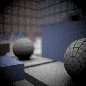
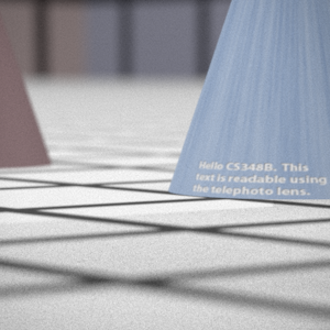
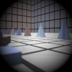
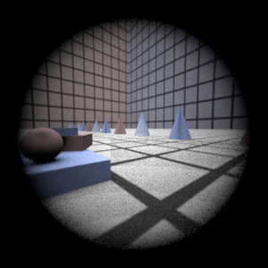
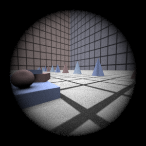
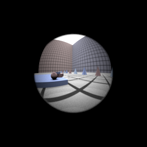
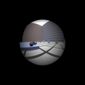
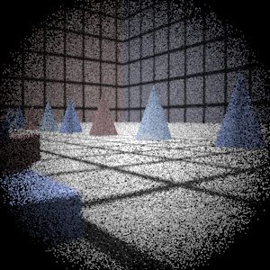
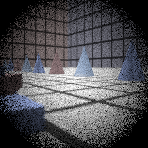
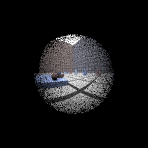
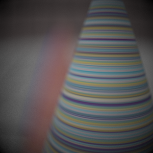
Final Images Rendered with 512 samples per pixel
|
My Implementation |
Reference |
Telephoto |
|
|
Double Gausss |
|
|
Wide Angle |
|
|
Fisheye |
|
|
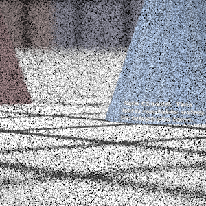
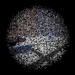
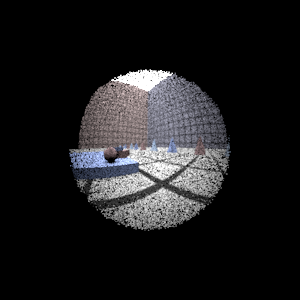
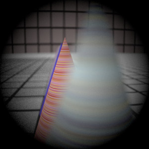
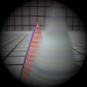
Final Images Rendered with 4 samples per pixel
|
My Implementation |
Reference |
Telephoto |
|
|
Double Gausss |
|
|
Wide Angle |
|
|
Fisheye |
|
|
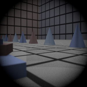
Experiment with Exposure
Image with aperture full open |
Image with half radius aperture |
|
|
Observation and Explanation
The f-number is given by the ratio of the focal length and the aperture. Once, we reduce the aperture to half, lesser number of rays pass through the entire ray system. As a result, the exposure decreases by 2 stops. As can be seen the simulation with half the aperture open produces an image with reduced exposure and thus is darker than the other one.
Autofocus Simulation
Description of implementation approach and comments
The Autofocus algorithm I used depends on the Sum Modified Laplacian(SML) as described in [1]. The autofocus zones are read in the files and SML is computed for them. The RGB values returned for each pixel based on the rays generated by Generate Ray are used to compute the SML. At first the RGB values were converted into intensity values using I = 0.212671f*r + 0.715160f*g + 0.072169f*b. Once these were found for each pixel in the zone, a window of 3X3 was used to find the gradients in the image using SML. The average of SML's of the entire zone was then found and was used to calculate the standard deviation of the zone. As an image with high gradients would have values away from the mean, a focussed image thus, will have a high standard deviation. This was used as the deciding criteria for the highest focus. Though SML not completely accurate, it gives a reasonable approximation.
A range of focusses were checked for their standard deviation. The range started from 0 100 at first with a step size of 10. After an optimum filmDistance was found, the range was narrowed to +/- 5 of the current filmDistance with a step size of 1 and again the standard deviations were checked. Finally, a step size of 0.1 determined the final filmDistance. Also, to avoid noise interplayiing with the focus calculations, the number of rays per pixel was increased. This implementation seemed quite slow and I added few optimizations to make it faster. At first, if the standard deviation went below a certain threshold(determined by the current maximum), I skipped the search beyond that.
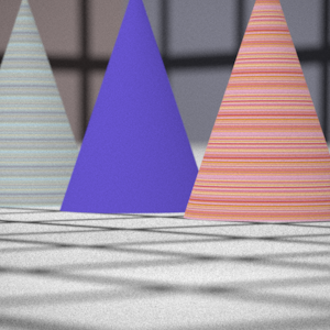
For multiple AF Zones, I introduced a mode flag which could be set from the pbrt file, to determine whether foreground or background has to be focussed. This determined which of the filmdistances obtained by the multiple Afzones have to be selected. For foreground, it would select the largest optimal filmdistance and for the background, it would select the closest. I obtained the image shown below as a result of the autofocus_test scene file. It worked for the foreground, but I tried hard to make it work for the background, but somehow it didnt work. It found the filmdistance at about 62mm, but didnt produce the correct image.
References: [1] Shree K. Nayar, Shape from focus System.
Final Images Rendered with 512 samples per pixel
|
Adjusted film distance |
My Implementation |
Reference |
Double Gausss 1 |
62.2 mm |
|
|
Double Gausss 2 |
39.5 mm |
|
|
Telephoto |
116.8 mm |
|
|
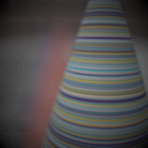
Any Extras
At 42.3mm
