Assignment 3 Camera Simulation
Tom Brow
Date submitted: 11 May 2006
Code emailed: 11 May 2006
Compound Lens Simulator
Description of implementation approach and comments
I represent the compound lens using a linked list of lens structs, each of which contains information about one lens surface or aperture stop. The surface of the element is represented as a pbrt Shape -- a Sphere for a lens surface, and a Disk for a stop -- and precomputed values for the refractive index ratio across the surface (i.e. n1/n2) and the cosine of the critical angle are stored as well. The compound lens structure also stores a Transform from camera space to lens space (and vice versa) so that the construction and intersection of lenses can all be done in lens space even if the lens is moved.
To generate a ray, the camera samples the aperture of the back element using ConcentricSampleDisk(), then initializes a ray through this point from the image sample point. It then traverses the linked list of elements, applying the vector form of Snell's Law (source: Wikipedia) at each surface in order. The ray is terminated and returned with weight 0 if it either (a) fails to intersect or (b) is totally internally reflected from any surface. Otherwise, the modified ray is returned with the weight given by Acos(theta)4/Z2, where A is the area of the aperture of the back element scaled by the area of the aperture stop (as a fraction of maximum aperture), Z is the distance from the film plane to the back lens, and theta is the angle between the original, unmodified ray and the normal to the film plane (source: Kolb).
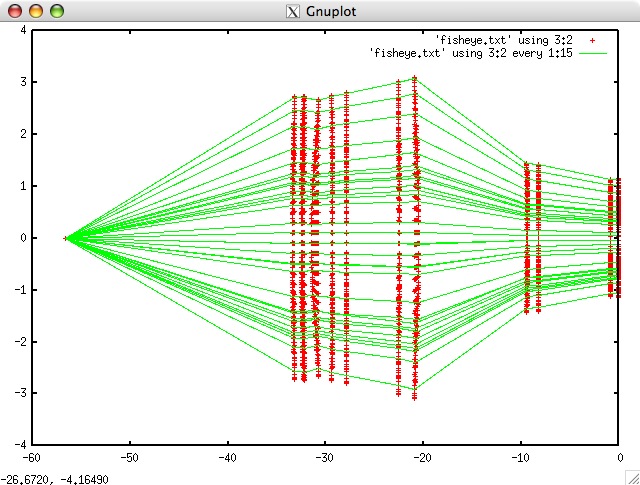
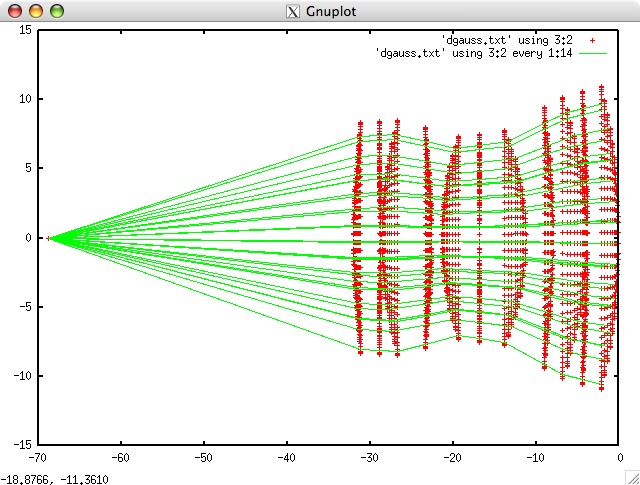
While testing by compund lens implementation, I found it useful to visualize the path of rays traveling through the lens. However, it would have been difficult to render the lenses and rays directly without a good deal of extra code. Instead, I had my program output every intersection that occurred inside the lens during ray tracing in 3D camera space coordinates, grouped by ray. Plotting these points in 2D and 3D space using gnuplot, I could visualize lens surfaces as clusters of intersections, and trace lines through groups of intersections to simulate rays. Here are plots for telephoto, fisheye, double gauss, and wide angle lenses.
I'm not sure why some of the unlit pixels in my output images come out white rather than black. It could be my EXR viewer/converter.
Final Images Rendered with 512 samples per pixel
|
My Implementation |
Reference |
Telephoto |
|
|
Double Gauss |
|
|
Wide Angle |
|
|
Fisheye |
|
|


Final Images Rendered with 4 samples per pixel
|
My Implementation |
Reference |
Telephoto |
|
|
Double Gausss |
|
|
Wide Angle |
|
|
Fisheye |
|
|


Experiment with Exposure
Image with aperture full open |
Image with half radius aperture |
|
|

Observation and Explanation
As expected, the brightness of the captured image decreases, and the depth of field increases slightly. Reducing the radius of the aperture by a factor of two means reducing the area of the aperture by a factor of 4, or decreasing the aperture by two f-stops (since one f-stop corresponds to a decrease in area by a factor of 2). Recall that the ray weighting formula takes aperture area into account.
Autofocus Simulation
Description of implementation approach and comments
I autofocused my camera using the RGB images rendered for the autofocus zones by the provided code. To keep things simple, I chose to measure focus using the Sum-Modified Laplacian operator from Nayar. I calculated the Modified Laplacian value for each channel for each pixel in the autofocus zone using a step value of 1, and ignoring those pixels within 1 of the zone border. I suspect that calculating the ML for each channel is important because it allows us to detect derviatives in areas that may have uniform total luminance, but varying color (like the texture of the striped cone). However, I did not experiment with simply converting the autofocus zone image to monochrome, so I can't be sure of this. The ML value for a pixel is the sum of the three channel ML values.
I did not bother calculating per-pixel SML values (as Nayar does, using a NxN neighborhood around each pixel), but instead simply summed the ML values of all non-border pixels to get an SML for the zone. Plotting that value over film distances from 28mm to 130mm, I found that there was always a disernable peak at the correct focal plane, but also that the SML increases steadily as film distance decreases, such that the global maximum value was usually at the minimum distance. Here are plots of SML over film distance for each of the three test scenes, using 16 samples per pixel to generate the render patches:

My somewhat inefficient solution for finding the appropriate local maximum was to try every film distance from 130mm to 28mm at 2mm intervals, stopping when a maximum SML was found that was not surpassed by any of the SMLs at the 4 (an empirically chosen number) succeeding intervals. In the test scenes, this method successfully identified the local maximum at the correct film distance.
Final Images Rendered with 512 samples per pixel
|
Adjusted film distance |
My Implementation |
Reference |
Double Gausss 1 |
mm |
|
|
Double Gausss 2 |
mm |
|
|
Telephoto |
mm |
|
|


Any Extras
...... Go ahead and drop in any other cool images you created here .....