Project Writeup : Sakura ("Cherry Blossom")
Team
- Tom Wang
- Priscilla Pham
Inspiration Images
|
|
|
|
Overview
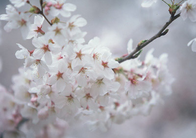
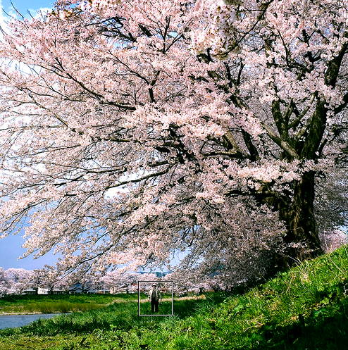
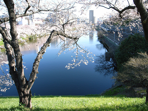
- Sakura trees (also known as cherry blossom trees) are among the most beautiful trees in nature and also present a worthwhile rendering challenge. In addition, we will procedurally model blossom petals by using an adaptation of the rose curve. Finally, we intend to employ subsurface scattering on the petals to capture the realistic details of softness and faint translucency.
Tree Overview
- I model the tree procedurally with a modified L-system (defined with probability distribution functions along each depth of recursion) using generalized cylinders. I then generate a per-cylinder displacement map based on the geometry of the cylinder to add natural bark perturbation, enhancing realism. Next, I overlay with a per-cylinder bump map to emulate the circular indents present in lentical bark. Finally, I texture map a cherry blossom bark onto each cylinder. I provide technical details of each component below.
Procedural Tree Generation - Tom
Source Code
L-system Background
- An L-system is a parallel string rewriting system, in which a simulation begins with an initial string called the axiom, which consists of modules, or symbols with associated numerical parameters. In each step of the simulation, rewriting rules—or productions—replace all modules in the predecessor string by successor modules. The resulting string can be visualized as a series of commands that link nodes, represent rotations, and distances between nodes.
Probability Distribution Function Implementation
- I model each part of the tree as generalized cylinders and control the look of the tree with the following parameters:
- Bottom radius
- Top radius
- Height
- 3D Rotation and Translation
- Initial radius fade (how much smaller the start radius of a sub-branch is)
- Final radius fade (how much smaller the end radius of a sub-branch is)
- Gnarling (overall displacement for next cylinder in link)
- Number of sub-branches
- Location of sub-branches Each cylinder is composed of a mesh of vertices in triangle strip format - these vertices are oriented as 'slices' (subdivisions around the main axis of the cylinder) and 'stacks' (subdivisions along the main axis of the cylinder). I am using a heavily modified gluCylinder() approach. Parameters are defined to be within certain ranges, depending on the level of branching, and are chosen with a uniform probability distribution function. For example, the trunk defines:
Trunk
- Trunk radius - [1.7, 2.0]
- Trunk height - [4, 5] * Trunk radius
- Initial Fade - [1, 1]
- Final Fade - [.8, .9]
- Branches - [2]
- Location of branches - [Trunk height]
Branch
- 1st Level Branch radius - Trunk's Top Radius
- 1st Level Branch height - [4, 12] * radius
- 1st Level Branch initial fade - 1
- 1st Level Branch final fade - [.3, .8] (varies linearly to branch height)
- Branches - [2, 3]
- Location of branches - [.95 * branch height, branch height]
Sub-branch
- Sub Branch radius - Previous branch top radius * initial fade
- Sub Branch height - [6, 12] * radius
Sub Branch initial fade - 1 (for level <= 3), [.8, .9] (otherwise)
Sub Branch final fade - [.1, .6] (for level <= 3), [.1, .35] (for level 4), [.3, .5] (otherwise)
- Branches - [2, 2], [3, 4], [2, 6], [1, 4] (for levels 3, 4, (5, 6), and 7)
- Location of branches - [.5, .95]
In order to generate the tree, I begin with the trunk and continue branching until I either reach a cutoff level (level == 7) or the branches become too small (radius < .01). This technique is implemented as described in Oppenheimer's paper [10]. A few more details involved adding discs to either end of the cylinder to make them closed cylinders, creating a probability distribution for arbitrary rotations in 3D space, sectioning 3D space so that each branch gets its own portion to try to prevent against branch intersection (a true intersection test would be nice, but too expensive), modeling the vertical inclination of trees as described in Weber's paper [11], and calculating PDF parameters to ensure the tree stays within a desired bounds (also mentioned in [11]). The images below demonstrate my tweaking of PDF parameters to match the desired ratios for realistic cherry blossom trees.
Basic Texture, No Branching
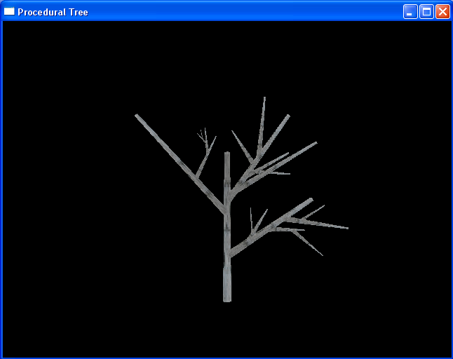
Basic Branching, Lighting
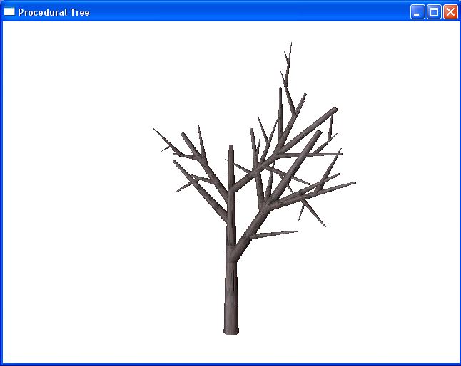
Model Leaves, Perspective
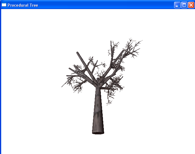
True Branching, Cherry Tree Properties
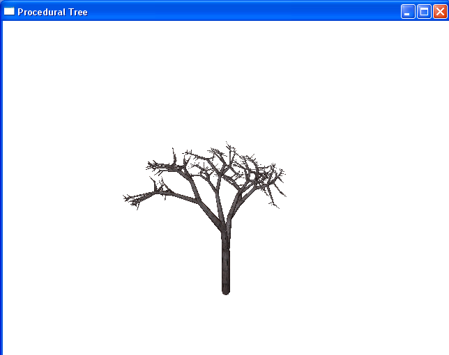
Gnarled Rotations, Proportional Trunk
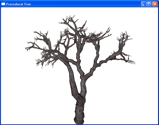
Smooth Gnarled, Reduce Leaf Noise
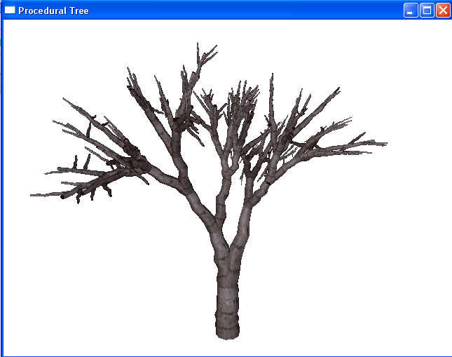
Increase Triangle Count, Decrease Sudden Knobs
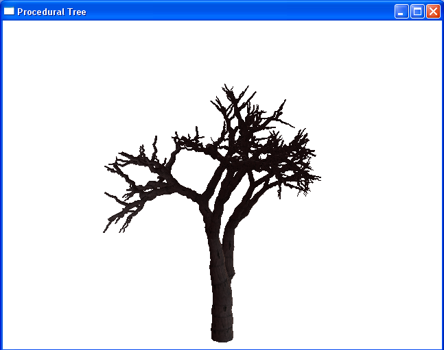
Procedural Bump and Displacement Mapping - Tom
In order to better simulate the natural bumpiness of trees in reality, it became important to introduce displacement maps to change the physical geometry of vertices on the generalized cylinders as well as bump maps to change lighting normals and emphasize 'rings' of depth indicative of lentical bark. I first attempted to implement this inside a vertex shader using a texture as the source for normals and displacement and soon discovered that I needed to know the geometry related to each vertex to achieve the desired effect. Displacing too much would make small branches look weird and displacing too little would affect the trunk.
Instead, I chose to solve this problem by creating procedural displacement maps per branch - these maps look like random noise ranging uniformly from [-branch_radius/4, branch_radius/4]. Also, I create procedural bump maps per branch - these maps look like different frequencies of horizontal lines, each row has a random probability of generating a line and probabilities for the offset and length of this line. When applied to the tree, the bump map looks like circular rings.
I intended to also implement procedural texture mapping in the same fashion but discovered that PBRT only takes a single texture as input for triangle meshes. This means that I could not achieve a per-cylinder effect as I had done prior (I used OpenGL to modify the vertices and surface normals before I output to PBRT) unless I created an extremely large texture and had each cylinder index into a different portion of the texture. I did not have time to implement this before the rendering competition and was forced to use a static texture of a cherry tree.
Below is a picture of the tree with displacement mapping.
Natural Bark Perturbation With Displacement Mapping
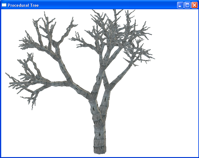
OpenGL Application for Rapid Prototyping - Tom
Since PBRT doesn't allow for camera controls in real-time without doing another rendering pass, I wanted a much quicker prototyping environment to tweak my many parameters. I opted to go with OpenGL and defined a fairly comprehensive application that allowed me to rotate, zoom, translate, change perspective, generate a new tree, and output to PBRT file at runtime. This turned out to save me a lot of time overall since small tweaks on PBRT were prohibitively slow. I ended up writing a quick file utility that would output an OpenGL triangle strip into a PBRT triangle mesh with normals, texture coordinates, and indices defined.
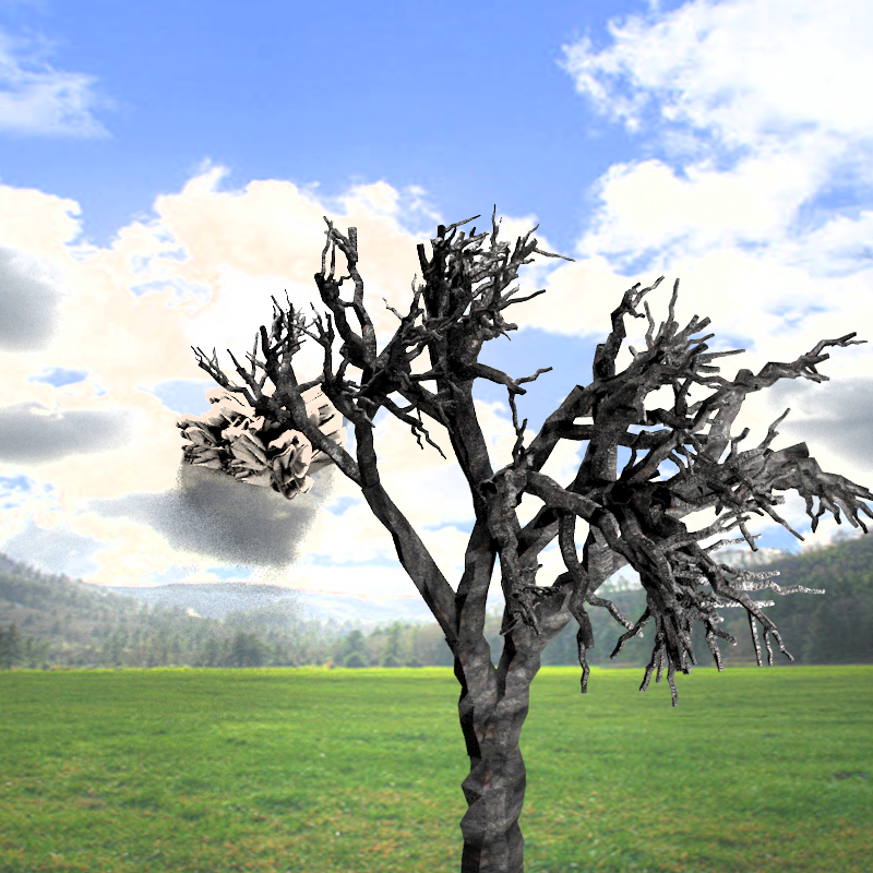
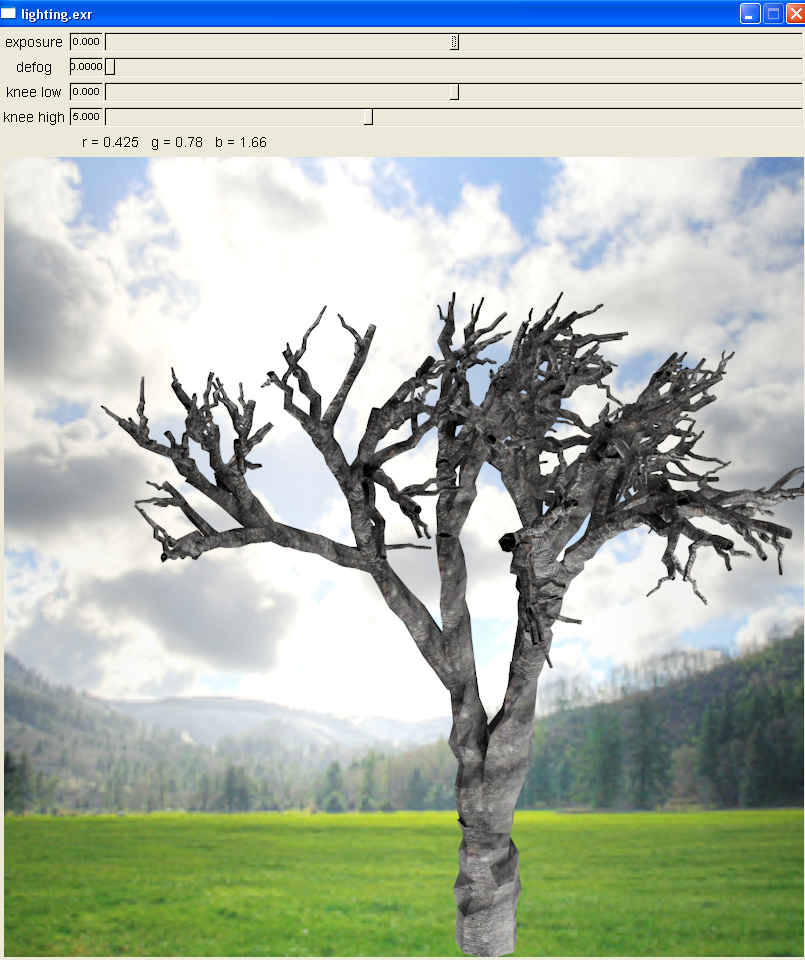
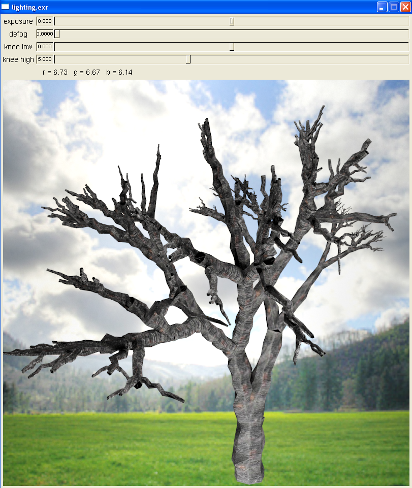
Finally, the last work left was to tweak the image, find a good tree model, and pick a backdrop.
Ninth Render (backdrop)
Ninth Render (different model)
Classic Plane Curves
Background
Prunus serrulata are dicots and possess five petals, five sepals, several stamen and a pistil.
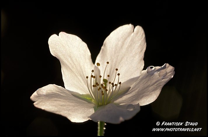
We observed that in this case that the beauty of nature coincides with the beauty of mathematics. More specifically, the shape and geometry of these blossoms can be recreated with curves defined in polar coordinates.
Blossom Geometry (Priscilla)
The blossom is constructed from plane curves that most closely resemble the shapes of the petals and sepals. The following is a diagram of the parts of a typical dicot:
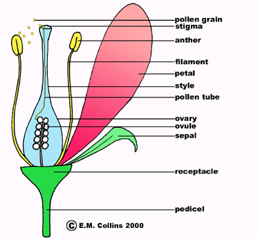
The shapes of the petals resemble cardioids:
Upload new attachment "cardioid.png"
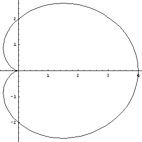
... and the placement of the petals are similar to the maxima of the 5 petal rose curve:
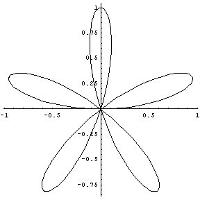
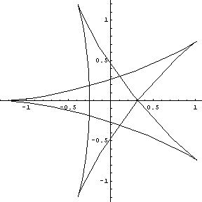
The star shape and positioning of the sepals resemble a 5 point hypocycloid :
This is a mathematica modeling of a single petal, with the commands used:
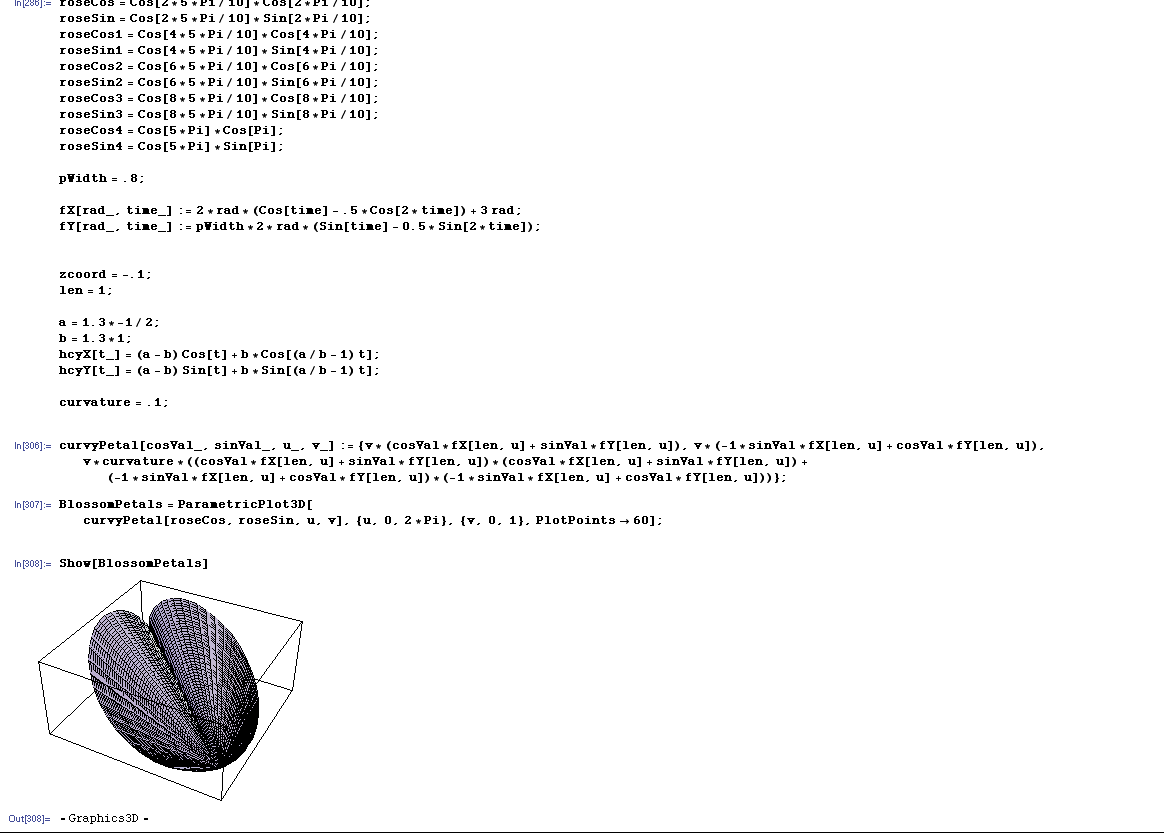
All petals together:
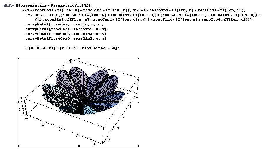
and then with varied sine and cosine noise added to the z-component as well as variance in curvature, so that the petals are not completely flat and emulate the imperfection in nature:

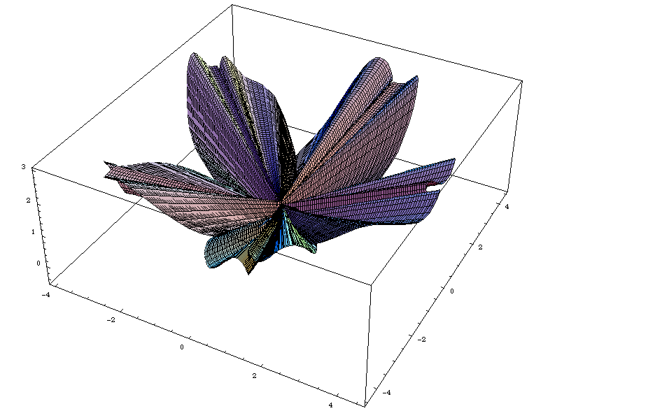
The petals are cardioids with the z-coordinate following the shape of a paraboloid to create the upcurving effect of the petals. The position of the petals around the center of the blossom are calculated according to those of the 5 petal rose curve. This final version of the model took more than an hour for Mathematica to render and would sometimes abort in the middle. If the increment step were decreased, the crinkles became sharp and jagged instead of smoothly curving. The final product was well worth the wait but the rendering effort was an unexpected roadblock.
The following is a Mathematica model of the sepals made of the hypocycloid with similar parabolic upcurving, plus the stem:
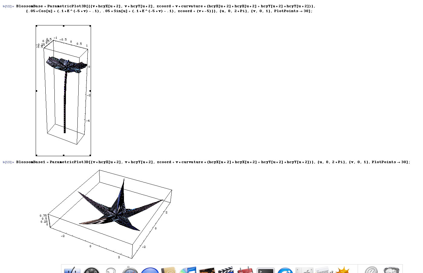
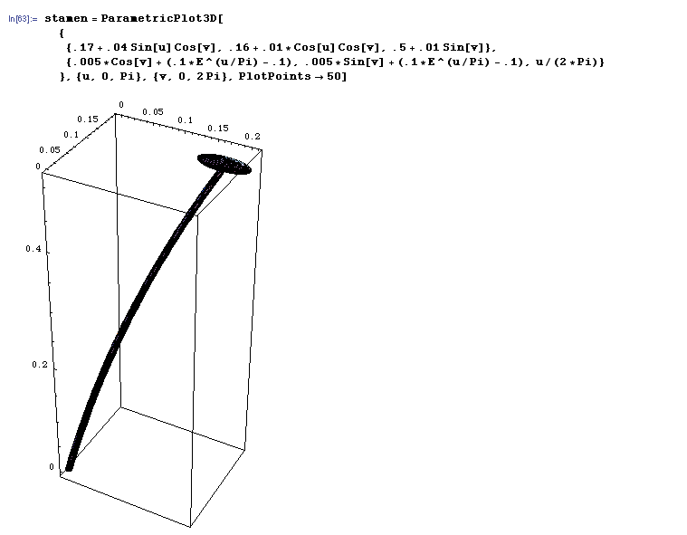
The pistil and stamen are relatively straightforward to generate, as they are just segments with ellipsoids at the end.
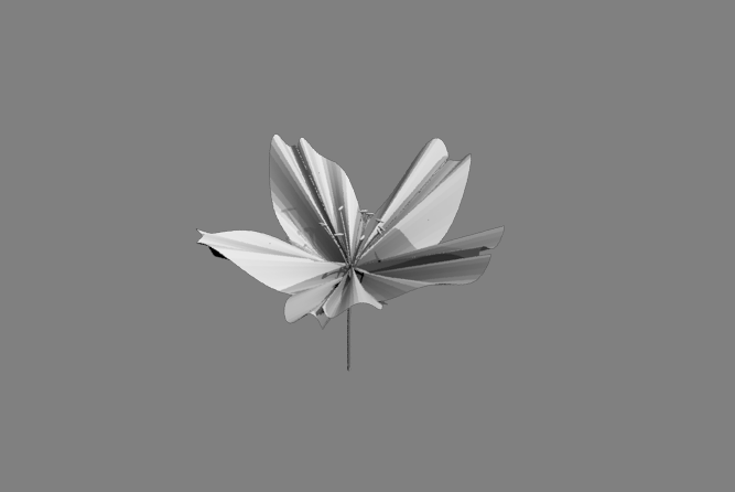
The following is a plain PBRT rendering of the final bare model:
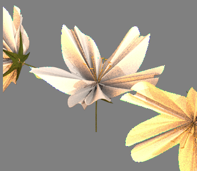
Here is one of the images where I experimented with color, texture, and environment map infinite lighting. Notice also a rotated version where the sepals at the base are displayed prominently:
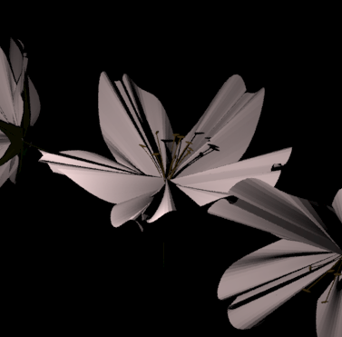
Here is some experimentation with "dramatic" spot lights. lt gave a poor effect, as spot lights usually give a harsh appearance:
Texture Mapping (Priscilla)
After petal generation has concluded, the plan was to generate randomized veins on the petal (all originating from the center) with a jitter transform, vertex noise, and/or Worley cellular texturing (procedural). According to one paper that this would have been based on, "The vein pattern for the petals is actinodromous venation, in which three or more primary veins diverge radially from a single point. Primary veins support sequences of secondary (lateral) veins, which may branch further into higher-order veins. The secondary veins and their descendants may be free-ending, which produces an open, tree-like venation pattern, or they may connect (anastomose), forming loops characteristic of a closed pattern. Tertiary and higher-order veins usually link the secondaries, forming a ladder-like (percurrent) or netlike (reticulate) patterngrid size in every simulation step, which precludes continuous simulation of growth. Vein segments are straight, and segments double in length in each growth step, which yields artificial-looking long straight lines running through the pattern." [7] This could possibly have been done with l-systems, although a different kind from the one used for the tree branches. Due to time constraints, however, this was not applied.
Subsurface Scattering (Priscilla)
Subsurface scattering (or SSS) is a mechanism of light transport in which light penetrates the surface of a translucent object, is scattered by interacting with the material, and exits the surface at a different point. The light will generally penetrate the surface and be reflected a number of times at irregular angles inside the material, before passing back out of the material at an angle other than the angle it would reflect at had it reflected directly off the surface. (Wikipedia)
Background
Rose petals are translucent and to achieve the realistic, silky, lifelike softness we must implement SSS. This may be achieved with the reflection model described in the paper by Hanrahan/Krueger. We will also study the structure and cellular layers of petals. So far, we have learned that two especially characteristic layers, such as upper epidermal cells which are dome-shaped and spongy cells which reflect much light, cause the unique appearance of rose petals.
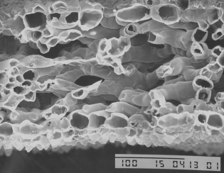
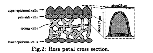 [9] Petals resemble thin surfaces, and their cross-sections can be described by open contours. We hope to apply this and other plant biology knowledge to enhance the appearance of the sakura petals.
Petal SSS
I wrote a new petal material plugin to PBRT, which added the BxDF per Hanrahan and Krueger [4]. I noted that in the diagram above of the cellular layers of petals was significantly less and thinner than the leaf diagram that the paper mentioned and took this as a justification of using the first order approximation method. The radiance is computed by summing the radiance from surface and subsurface scattering, and the transmitted radiance from the sum of the radiance from absorption and subsurface scattering. From these values and the Fresnel coefficients, I calculate the BRDF and the BTDF. I used an index of refraction of 1.37 which is reasonable for epidermis of skin.
For the phase function I used the Henyey-Greenstein approximation given in the paper:

Backscatter radiance:

Forward scatter radiance:
 :
:
Foward scatter ignoring singular values:

For setting the initial specular and diffuse values I used a color picker in The Gimp on the model image. What could have been done further was to look into the properties of the layers given in the Kotani[8] paper and applied the algorithm in a similar fashion to the leaf in the Hanrahan/Kreuger[4] paper.
Final Single Sakura Blossom
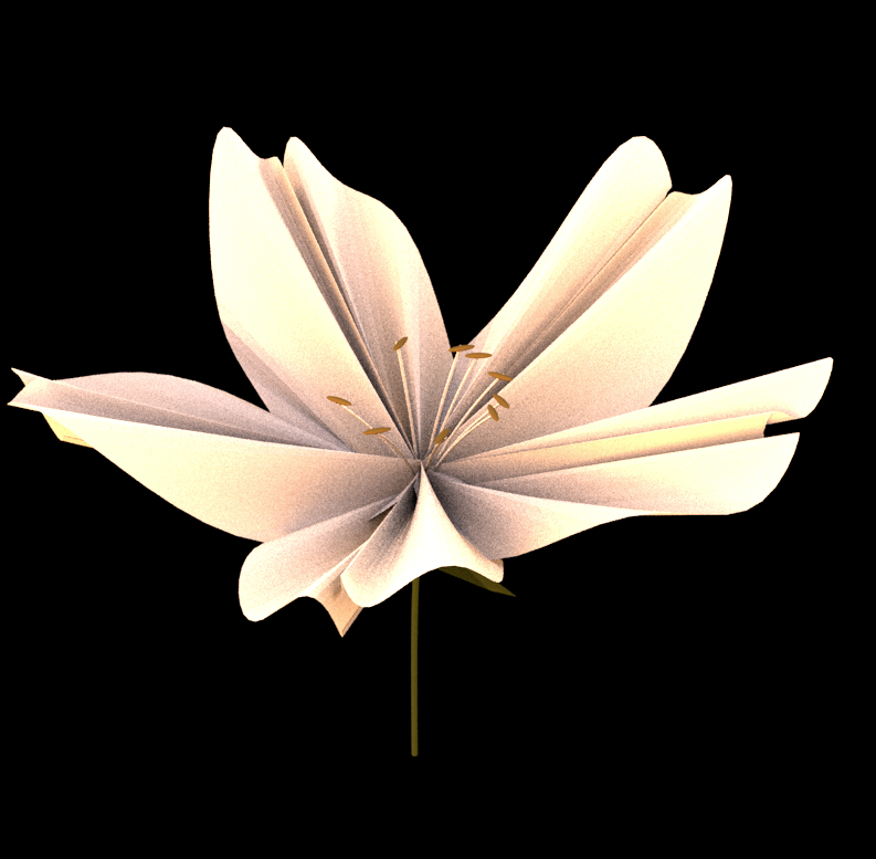
One Blossom Next to Tree
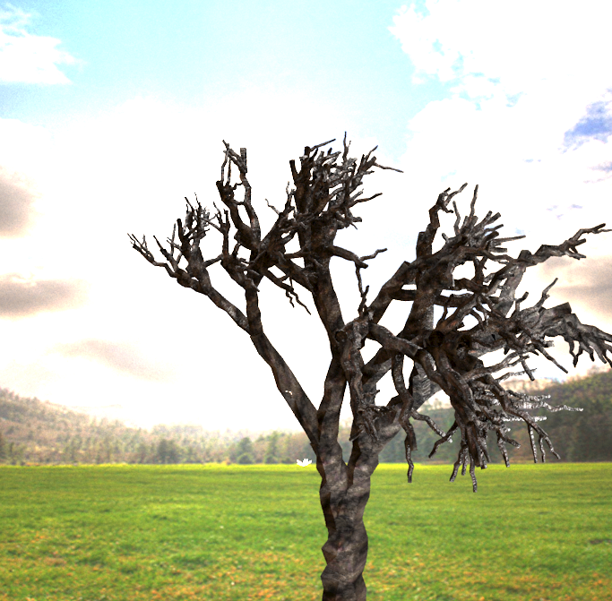
Final Image
