Physically Realistic Volume Rendering
Group Members
James Hegarty
Qiqi Wang
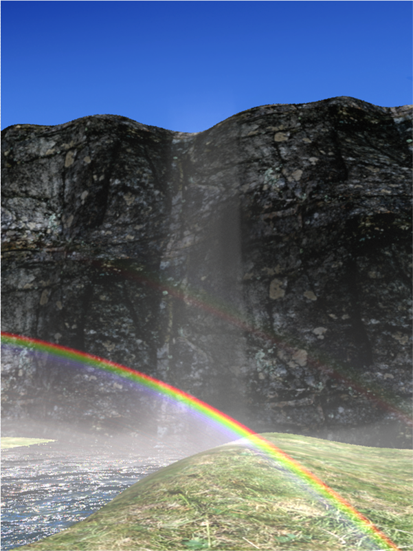
Final Image
Added / Modified Code
Overview
In this project we rendered a scene based on a physically accurate light scattering model for volumetric materials made up of transparent particles. Special effects such as rainbows can be also rendered with this model. In order to accurately model the distribution of volume materials in complex geometry, a physically based fluid calculation must be performed, resulting in an unstructured mesh. A ray tracing algorithm for unstructured meshes was developed, and light reflection and scattering models from these volume materials was built.
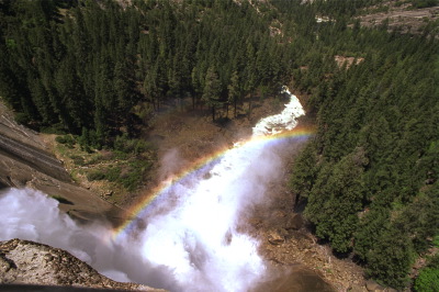
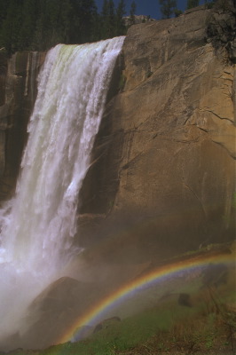
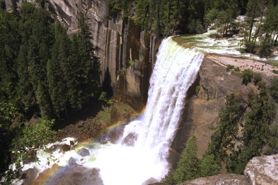
The following pictures are from www.ImageMontage.com , I believe they are taken at the Nevada fall in Yosemite. The waterfall and rainbow is the type of things we want to render.
|
|
|
Modeling of volume material distribution (Qiqi Wang)
In order to model the distribution of volume materials accurately, we will use the commercial flow solver Fluent. In the waterfall scene, we use commercial Computational Fluid Dynamics software Fluent 6.2 to calculate the flow of air around the waterfall, as well as the density of water drops in the air. The size of the mesh is 1000 ft by 1000 ft by 6000 ft, the waterfall alone is 100 ft tall. The following pictures demonstrates the mesh generated for the Computational Fluid Dynamics calculation. The first picture shows the surface mesh, the second picture shows the volume mesh on the symmetric section plane.

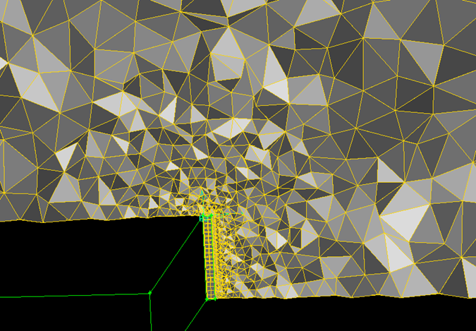
This is a typical unstructured mesh used for Computational Fluid Dynamics calculation around complex geometry. First of all, tt has huge mesh size variation. The cells inside and near the waterfall is small, and the cells away from it is ten thousand times larger in volume. Also, it has three different types of cells. Inside the waterfall, octohedral cells are used; away from the waterfall, hexahedral cells are used; pyramid cells are used as a layer between octohedral cells and hexahedral cells.
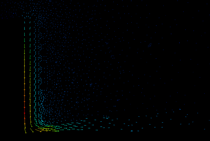
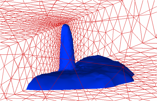
The velocity field and the density of water drops are computed by Fluent 6.2, a most up-to-date commercial Computational Fluid Dynamics software. The small volume in the middle of the step is used to model the water fall, and the rest of the volume is used to model the air. The flow field is calculated using incompressible Navier-Stokes equation with k-e turbulence model. We model the driving force by the flow of water inside the waterfall as a constant downward source term in the momentum equation. This source term drives the flow field in the entire volume. We model the floating water drops in air as transporting and reacting chemical species, whose density is also solved by Fluent 6.2. Inside the waterfall volume, the water drop density is generated in a constant rate. In the rest of the volume, the water drops evaporates into vapor and convects away from the waterfall. The following two images shows the flow field on the symmetric cut plane and the isosurface of 20% of the maximum water drops concentration. Our rainbow image is rendered based on this calculated density field of the water drops.
Ray tracing through unstructured mesh (Qiqi Wang)
In PBRT, we added a file volumemesh.cpp in the volumes folder to deal with unstructured mesh ray tracing. The bulk of this code is four classes (VolumeMesh, Mesh, Cell, Face) and mesh file I/O routines. In our data structure of storing the mesh, each face is an object of the Face class, which stores position of all its vertices, its face normal and two pointers to its adjacent cells; each cell is an object of the Cell class, which stores pointers to all its faces and the water drops density in the cell. The definition of the classes are as follows:
   1 struct Face {
   2         int id;
   3         vector<Point> vertices;
   4         Cell *c0, *c1;
   5         Vector faceNormal;
   6         void CalculateNormal();
   7         bool Intersect( Point o, Vector d, float& t ) const;
   8         Point Center() const;
   9 };
  10
  11 struct Cell {
  12         int id;
  13         vector<Face*> faces;
  14         vector<float> scalars;
  15         bool Intersect( Point o, Vector d, float& t0, float& t1,
  16                         Face*&f0, Face*&f1 ) const;
  17 };
Both Face and Cell class have an Intersect method, which determines whether a given ray intersect with the Face / Cell, and calculate the intersection point(s). To calculate the intersection point of a ray with a face, we just need to compute the intersection of the ray with the face plane, which can be done in 2 dot products and 1 division. Determination of whether the ray intersects with the face is much nore difficult. Our algorithm is to calculate the total angle of the face edges with respect to the ray. If the total angle is plus or minus 2*pi, then the ray intersects with the face; if the total angle is 0, then the ray does not intersect with the face. The total angle cannot be any other value. For robustness reason that will be explained later, we project the face onto a plane that is normal to the ray before calculating the total angle. It takes roughly 4 dot products, 1 cross product, 4 normalization and 1 arctan2 operations for each edge of the face to determine intersection. To calculate the intersection points of a ray with a cell, we test intersection of the ray with all its faces. Only 0 or 2 faces should have an intersection with the ray assuming the cell is convex. The code for the two Intersect methods are:
   1 bool Face::Intersect( Point o, Vector d, float& t ) const {
   2     const float EPS = 0.0001;
   3     // calculate intersection point and t
   4     float total = Dot( d, faceNormal );
   5     float sect1 = Dot( vertices[0] - o, faceNormal );
   6     if (total == 0) return false;
   7     t = sect1 / total;
   8     // calculate total angle around itersection point
   9     float angle = 0;
  10     for (int i=0; (size_t)i<vertices.size(); i++) {
  11          int ip = (i+1) % vertices.size(); // next vertex
  12          Vector arm1 = vertices[i ] - o;
  13          Vector arm2 = vertices[ip] - o;
  14          // project to the foot of the ray
  15          Vector unitd = Normalize(d);
  16          arm1 -= unitd * Dot(arm1,unitd);
  17          arm2 -= unitd * Dot(arm2,unitd);
  18          // right on top
  19          if (arm1.Length() == 0 || arm2.Length() == 0) return true;
  20          // compute the angle of this side
  21          arm1 = Normalize(arm1);
  22          arm2 = Normalize(arm2);
  23          float sine = Dot( Cross(arm1, arm2), unitd );
  24          float cosine = Dot(arm1, arm2);
  25          float side_angle = atan2( sine, cosine );
  26          // add to the total angle
  27          angle += side_angle;
  28     }
  29     // intersect within the face if the total angle is +- 2*PI
  30     if (2*M_PI-EPS < fabs(angle) && fabs(angle) < 2*M_PI+EPS)
  31         return true;
  32     // otherwise the total angle must be 0
  33     else if ( fabs(angle) > EPS ) {
  34         Error("\nTotal angle equal to %f in intersection\n", angle);
  35         cout << "o = " << o << " d = " << d << "\n";
  36         for (int i=0; (size_t)i<vertices.size(); i++) cout << vertices[i] << endl;
  37         return false;
  38     }
  39     return false;
  40 }
  41
  42 bool Cell::Intersect( Point o, Vector d, float& t0, float& t1, Face*&f0, Face*&f1 ) const {
  43     t0 = 1E10; t1 = -1E10;
  44     bool iIntersect = false;
  45     // find intersection with all faces.
  46     for (int i=0; (size_t)i<faces.size(); i++) {
  47         float t;
  48         if (faces[i]->Intersect( o, d, t )) {
  49             iIntersect = true;
  50             if (t <= t0) { t0 = t; f0 = faces[i]; }
  51             if (t >  t1) { t1 = t; f1 = faces[i]; }
  52         }
  53     }
  54     if (iIntersect && t0 == t1) {
  55         if (f0 != f1) {
  56             // decide which face is more on the side of the ray direction
  57             if (rand() > rand()) {
  58                 Face* ff = f0;
  59                 f0 = f1;
  60                 f1 = ff;
  61             }
  62         }
  63         else {
  64             Error("\nt0 == t1 and f0 == f1 in Cell::Intersect, t0=%f, t1=%f\n", t0, t1);
  65             cout << "CellId = " << id << " o " << o << " d " << d << endl;
  66             cout << "f0 = " << f0->id << " f1 = " << f1->id << endl;
  67             return false;
  68         }
  69     }
  70     return iIntersect;
  71 }
The Mesh class manages all the cells and faces. It also manages a 'Current Point' and 'Current Cell' that can be efficiently moved by tracing a ray through the mesh volume. The ray tracing algorithm through the volume mesh is implemented with the MoveTo method of this class.
   1 class Mesh {
   2 public:
   3         Mesh( string filename, int numScalars );
   4         Point CurrentPoint() { return currentPt; }
   5         const Cell* CurrentCell() { return &cells[currentCell]; }
   6         bool MoveTo( Point target, vector<const Cell*>& trajectory, vector<float> t0, vector<float> t1 );
   7         BBox bbox() const { return BBox(p0, p1); }
   8 private:
   9         Point currentPt;
  10         int currentCell;
  11         int numFaces, numCells;
  12         Face* faces;
  13         Cell* cells;
  14         Point p0, p1;
  15         void CalculateBBox();
  16 };
  17
  18 bool Mesh::MoveTo( Point target, vector<const Cell*>& trajectory, vector<float> vt0, vector<float> vt1 )
  19 {
  20     const Cell *c = CurrentCell();
  21     Point  o = currentPt;
  22     Vector d = target - currentPt;
  23     float t0 = 0, t1 = 0;
  24     int iter = 0, maxiter = 10000;
  25     while (c != NULL) {
  26         if (iter++ > maxiter) break;
  27         Face *f0 = NULL, *f1 = NULL;
  28         bool isect = c->Intersect(o,d,t0,t1,f0,f1);
  29         if (!isect) {
  30             Error("Failed to find intersection for cell %d\n", c-cells);
  31             cout << "o = " << o << ", d = " << d << "\n";
  32             return false;
  33         }
  34         assert( f0!=NULL && f1!=NULL );
  35         // save trajectory
  36         trajectory.push_back(c);
  37         vt0.push_back(t0);
  38         vt1.push_back(t1);
  39         if (t1 >= 1) break;
  40         // move to next cell
  41         if (f1->c0 == c) c = f1->c1;
  42         else if (f1->c1 == c) c = f1->c0;
  43         else
  44             Error("Mesh structure error detected in Mesh::MoveTo, Face %d with Cell %d\n", f1-faces, c-cells);
  45     }
  46     if (iter > maxiter) {
  47         Error("Mesh::MoveTo, maximum iterations %d reached.\n", maxiter);
  48         return false;
  49     }
  50     // modify current point
  51     if (c != NULL) {
  52         currentCell = c - cells;
  53         currentPt = target;
  54         return true;
  55     }
  56     // return value indicates whether we are able to move to the point
  57     else return false;
  58 }
The VolumeMesh class is a subclass of DensityRegion. It manages a Mesh class. It overrides the Density function and returns the density of any given point by use Mesh::MoveTo to move the 'Current Point' to the target point and return the density of the 'Current Cell'.
   1 float VolumeMesh::Density(const Point &Pobj) const {
   2         if (!extent.Inside(Pobj)) return 0;
   3         vector<const Cell*> trajectory;
   4         vector<float> t0, t1;
   5         if (mesh->MoveTo( Pobj, trajectory, t0, t1 ))
   6                 return trajectory.back()->scalars[0];
   7                 // return 1;
   8         else return 0;
   9 }
Finaly, the mesh file I/O routines are used in the constructor of Mesh class. It counts the number of cells and faces in the mesh, allocates memory space and reads the file content into our data structure.
Robustness Issues
In rendering each image, millions of rays sent into the volume mesh, and each ray intersect with thousands of faces and cells. Because of the huge number of intersections, extremely rare situations can occur. Rays that goes right through an edge creates two numerical problems: (1) Rays that goes right through an edge of a cell might be found to intersect with 1 or 3 faces of that cell. (2) The two intersect points of a cell can be two close to determine which is farther. Using double precision numbers instead of single precision numbers reduces the number of such numerical problems, but cannot solve them completely. In order to deal with that, we need to tweak the algorithm. First of all, when calculate the total angle around the ray, we project the face into a plane that is orthogonal to the ray. This makes the calculated angle of each edge with respect to a given ray independent of the face. Also, when the two intersection points are close, we use a randomized algorithm to determine which face is farther away in order to prevent dead lock.
Verification of ray tracing algorithm
The following three images are rendered to verify that we have a correct unstructured mesh ray tracing algorithm. In the first image, we set the light emmision factor to be constant within the entire volume. The rendered result matches the shape of the mesh in the previous section. In the second and third image, we set the light emmision factor to be proportional to the water drops density calculated by Fluent 6.2. We see the shape matches the isosurface of waterdrops density shown in the previous section.
|
|
|
Visual Properties of Waterfalls
There were multiple visual effects that we wanted to capture in our waterfall rendering. First, we wanted to create a physically correct Rainbow model. Second, we wanted to simulate the effect of light bouncing around in the volume of water particles to create the cloudlike appearance of the water. Volumes of water particles behave differently from other type of particles because in an ideal situation they are clear, and thus do not either emit or absorb light. We wanted to create a model that correctly accounted for this.
Rainbow Physics
The rainbow implementation proved to be relatively straightforward. We first consulted Greenler's book, Rainbows, Halos, and Glories to determine the physical basis for rainbows. Essentially, as a light ray enters a water drop, it bounces around in the drop multiple times, each time reflecting part of the light back into the drop and refracting part of it out of the drop. The refracted light obeys snell's law, and the reflected light obeys the reflection law. The mix between reflected and refracted light depends on Fresnell's reflection law.
The image below shows an example of a single ray interacting with the drop:
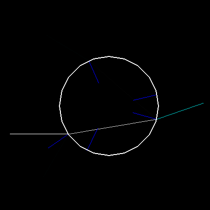
If all the light that enters the drop from one direction is considered, then due to the geometry of a perfectly spherical drop, a visually significant amount of light is focused at 42 degrees, creating the primary rainbow, and a secondary band appears at 51 degrees, creating a secondary rainbow.
The image below shows a record of all of the rays the leave the drop, if all of the rays that enter the bottom half of the sphere are considered. The peak areas where rays accumulate can be seen. Note: in reality, the light distribution would be like this picture, but mirrored across the horizontal axis. We're only considering half the rays in this picture to show the individual peaks.

Snell's law depends on the refraction index of the medium that the light is refracted through. The refraction index is slightly different for different wavelengths of light. Due to this effect, a colored rainbow is seen: the areas of focused light seen above is located at slightly different angles for different wavelengths, thus creating the familiar bands of color.
Because of the nature of how light rays interact with individual water drops, the rainbow is seen by the viewer. At an angle of 42 degrees between the light (assumed to be directional, like the sun) and the viewer, light rays are colored based on the properties of water drops explained above.
Rainbow Implementation
As the physics behind rainbows was well understood, all that remained was to alter the the volume integrator to include this effect. A simple sphere ray tracing program was written (attached below) that sent many rays through a sphere. It is straightforward, and is based on the physics above. Huibers created a sufficiently accurate approximation of the wavelength dependence of the refraction index based on physical measurements that we used in our implementation. The script accumulates the light from a large number of rays into a table indexed by the cosine of the angle between the light that entered and the light that exited. It then exported this table in a format readable by a C++ compiler (data.hpp, attached at top of page).
In order to deal with the wavelength dependent effects, the table was exported with the rays traced at 20 different wavelengths. In all rainbow code, calculations were made at these twenty wavelengths, and then converted to XYZ color using the CIE matching functions in the Spectrum class. This is not the most efficient method by far, but it was done to maximize flexibility.
The single scattering integrator was modified (rainbow.cpp, below) to use the rainbow table lookup to modulate the light that went from the light to the eye. To allow flexibility, the integrator was also modified to accept a virtual light position and rainbow brightness in the pbrt scene file. This is not physically correct, but for the purpose of producing our image it was expedient. A version based on the actual angle between the light and camera could easily be created. Directional light source would be required, as other light sources would cause multiple angles between the light and the eye to contribute to the same pixel in the image, bluring the rainbow to the point that it wasn't noticeable.
Code: drop.lua
Note: this script requires the freeware Baja Engine (http://www.bajaengine.com) to run.
Multiple Scattering with Path Tracing
While our single scattering based integrator was successful at producing rainbows, we wanted to accurately simulate the effect of light entering our volume of particles and interacting the the transparent particles before it reached the eye. To do this, we implemented path tracing based multiple scattering integrator.
Each ray that enters a volume region is simulated to walk through the region at a step distance provided by the user. At each step, the ray randomly either continues straight, or bounces off in a random direction, with a probability determined by the transmittance of the region through which it will travel in the next step. This corresponds to the physical concept of a light ray having traveling through space, and either continuing straight or being deflected based on whether it actually hit a water particle or not. If the particle is deflected, the color that the ray contributes is modulated using the drop rainbow table calculated using the method in the section above, based on the angle between the incident and refracted ray. Because a large number of the possible angles don't contribute a significant amount of light, importance sampling was used here to send more rays in the regions that contributed more light. Importance sampling here was based off the Distribution1D class implemented in infinitesample.cpp. It can be considered to be one dimensional, because the value only varies in one axis; the other axis is chosen randomly with a uniform distribution.
In order for the path tracing to be unbiased, each ray is weighted based on its probability of it actually occurring. Each step is calculated to have a certain probability, and this probability is multiplied by the weight of all past probabilities, because as a ray proceeds through the volume it becomes less probable that this specific ray would actually contribute to the scene. Specifically, each step is weighted by a factor of 1/(4pi)l, where l is the length of the step size. This is based on the derivation for surface path tracing found on page 746 of the PBRT book. For path tracing, a ray is weighted by the inverse of all possible rays could occur. In our case, all rays that could occur at a certain point in the volume come from an area of 1/(surface area of a unit sphere) = 1/4pi. Because we may want to consider spheres of different sizes, we change our weight to be 1/(4pi)l, based on geometry. For example, a sphere of radius 3 would have the probabily of 1/(4pi)^3, because it is essentially the probability of three unit sphere in succession. To further verify this formulation, it is also correct in the limit: as the sphere considered becomes infinitely large, the probability of a ray coming from that distance approaches zero, and as the sphere becomes infinitely small, the probability approaches 1.
The light source is an imaginary light source given as a parameter to the integrator; the implementation doesn't use the built in PBRT light sources as an optimization. The imaginary light is specified using a source point and direction. This forms an infinite planer light, and any path that crosses this plane is considered terminated. This is not physically correct, but it was useful for practical purposes and the implementation could be extended to use PBRT's light sources, at the expense of considerably more variance. The implementation has a maximum path size given by the user in order to prevent infinite loops in extreme cases. Rays that never make it to the light are ignored, and the final weighting of rays is altered so that they don't introduce bias, because rays that don't come from the light obviously aren't significant and should be ignored.
In order to retain the rainbow effect, we added a parameter in the integrator to bias the particles towards bouncing a ray directly at the light. This is not physically correct, but in order for the rainbow effect to the better controlled for artistic reasons, this is desirable.
Below is an image of a smoke dataset produced by Ron Fedkiw rendered with the light to the side using our integrator to show that it works properly. Note: the angle of view isn't wide enough to produce rainbows so they do not appear.
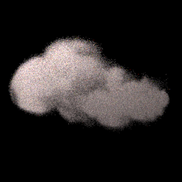
Compare this with the single scattering version:
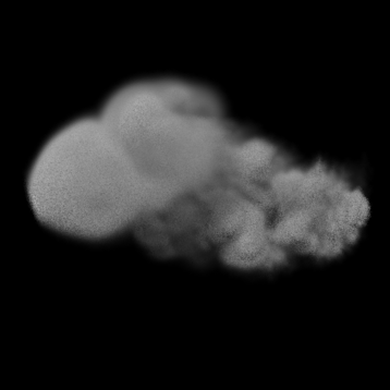
In the end we decided not to use this technique in our final image. In our image, the light is behind the camera, because this is when rainbow occur. Lit from behind the camera, the multiple scattering volume looked very similar to the image produced by the single scattering integrator with the high frequency information removed. As our volume data didn't include much high frequency information, we didn't find this difference to be significant. In addition, due to the complexity of our volumetric data set, we weren't able to produce an image of sufficient quality to actually see much of a result from the multiple scattering integrator in our final scene, due to the slow speed of path tracing. Indeed, we were never able to produce an image that showed much more than random noise, so none of these images are included. See the comparison of the single scattering vs. multiple scattering lit from behind the camera below:
Single Scattering:
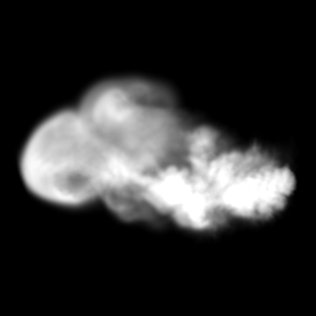
Multiple Scattering:
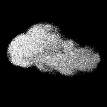
Further obvious work on this would be to create a photon mapping based version of this integrator and try to use it in the actual image.
Other, Misc Work
The background was modeled in Softimage XSI. As there is no direct path from XSI to PBRT, we exported from XSI to obj format and used the wavefront editor written by Mark Colbert (http://www.cs.ucf.edu/~colbert/mayapbrt/goodies.html). Unfortunately, the exporter has a bug that results in the normals not being imported correctly. We weren't able to fix this problem, so we just had PBRT generate default normals for the objects. This leads to visible facets in the object because the objects aren't smooth. To counteract this, the objects were subdivided heavily.
The Sky, Rock, and Grass textures were from photographs. The Water was a glass material with a Perlin noise bump map applied.
References
Greenler, Rainbows, Halos, and Glories Huibers, Paul. Models for the wavelength dependence of the index of refraction of water. Applied Optics, Vol. 36 No. 16, June 1997. Humphreys, Greg and Pharr, Matt. Physically Based Rendering.
