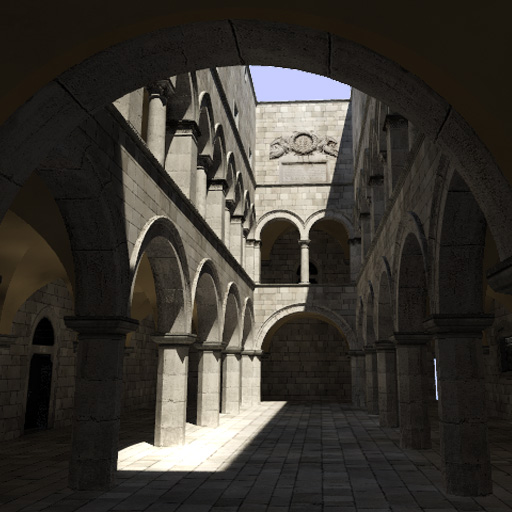
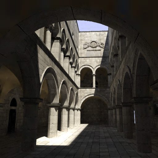
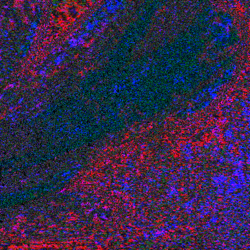
Figure 2 - Spatially
adaptive sampling (result above right) successfully captures this detailed
synthetic scene (original above left) with slightly under 50% compression
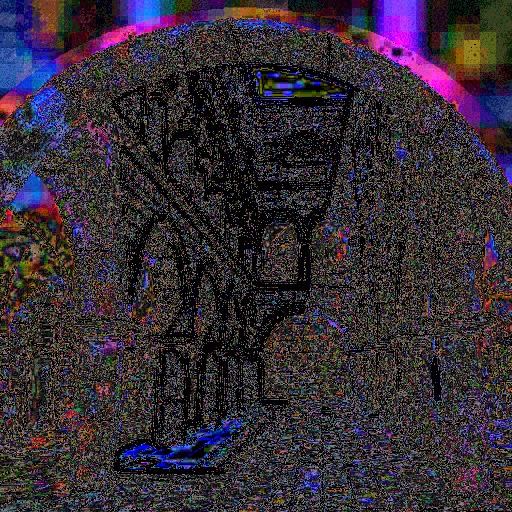
at an accuracy tolerance of 10. The exaggerated difference image demonstrates
that the relatively simplistic, hardware-implementable approach effectively
samples the high contrast, high frequency edge regions which appear black
due to their lack of error. Through most of the image, the differences
appear as random noise within the the 10 level tolerance. This noise corresponds
to loss of accuracy to randomness in the highest frequencies -- an effect
which is hardly perceptible. In the dim, lower frequency, more smoothly-varying
regions of the image, the sampler throws away the most data, generating
the most error around the rim of the near archway.
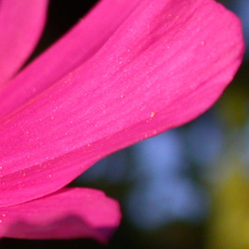

Adaptive sampling (result above
right) successfully captures this multi-frequency photographic image (original
above left) with over 70% compression at an accuracy tolerance of 10 levels.
This image, shot at 3 megapixels in macro on a Nikon Coolpix 995, is particularly
advantageous to the sampler as its nearly singular depth of field leaves
much of the image out of focus, with small regions of fine, high frequency
detail. The difference image confirms that the sampler aggressively subsamples
the severely defocused background. Still, it successfully creates a high
quality image which is barely distinguishable from the source. In direct
comparison to the original, it exhibits slight blockiness from the interpolation
in the clearly circular regions of confusion in the far background, as
well as some in the slightly defocused far midground of the flower petals.
However, the image taken on its own, its subsampling artifacts are imperceptible.