In our project proposal, we presented a
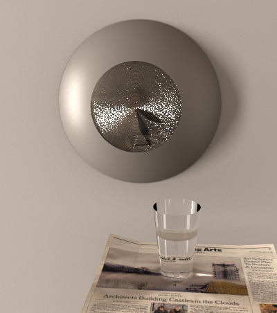
scene photographed from real life - a simple still life composed of a shiny
wall clock, a newpaper, and a glass of water. The scene had a number of
visual features that we wanted to model, as previously discussed in our
proposal. In this document, we will present a brief overview of the
modifications and extensions that we made to lrt in our
attempt to model this scene and simulate global illumination within it.
A small sample rendering is shown in Figure 1. Several images are still pending.
Figure 1: Sample rendering (larger copy)
The remainder of this document is divided into two sections, one by each of the collaborators on this project. These sections describe the individual contributions of each author.
We modeled the scene in a hand-crafted .rib file using existing lrt primitives. A heightfield was used for the newpaper to approximate the slight upward curl in the upper left corner. The scene uses area lights extensively - the entire hemisphere in front of the wall plane is filled with area lights! While the shiny elements of the scene are what first made it interesting to us, effectively modeling the diffuse illumination proved challenging. The soft shadows and the gradual variation in illumination over the wall surface are important to the realism of the scene, and provided a real workout for our ray tracer.
We acquired an environment map of the scene's surroundings - Mike Cammarano's living room - by photographing a small mirrored ball placed in the center of the real scene (with the clock and glass removed). Initially, we hoped that it might be possible to use this environment map directly as a representation of the scene's surrounding lighting conditions. Our attempts to do this were not successful, however. There seem to be two major difficulties with this idea: insufficient dynamic range in the environment map image, and inadequate methods for sampling the environment map as a light source. Both these issues could have been resolved, but we opted instead to use a simple approximation of the scene lighting composed of area lights, and focus on other aspects of the illumination problem.
Note, however, that the environment map has been put to use. It is texture mapped onto a sphere surrounding the scene, and can be seen in reflections off the clock's glass face and (in principle) off the glass of water, although little reflection is discernible in the latter.
The most challenging extension to lrt that we
undertook was the addition of photon mapping to reproduce the
caustic effects within the scene. The most perceptually significant
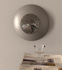
caustic in the original scene can be observed in the base of the glass,
which should appear brightly lit (see the original scene photograph), but which is black in an image
ray-traced without caustic effects. (See Figure 2).
Figure 2: A glass of water, rendered using simple monte carlo ray
tracing (left) and with the addition of photon mapping to reproduce
caustics (right).


Our original scene didn't feature any significant caustic effects other than the illumination of the bottom of the glass. However, we showed in a supplemental photograph that the introduction of a point light source cast interesting caustics (Figure 3 of our project proposal). In our rendering, we chose to introduce an additional light source to the scene to create this exaggerated caustic, allowing us to show off the photon mapping. Alas, even with this addition, cool photon mapped caustics still occupy fewer than 1% of our final scene's pixels. Look close!
Now, a brief discussion of implementation. Tracing photons through
a scene is similar to tracing rays. However, every
time a photon interacts with a surface we must be able to choose a single
direction to reflect or transmit the photon from the appropriate scattering
distribution. To allow this, we extended the BRDF classes needed for the scene to
incorporate this extra functionality. For example,
ScatteringMixtures can be sampled with a photon, randomly
choosing one of the mixture's child BRDFs with some weighted probability,
and using that child BRDF to choose the photon's reflection.
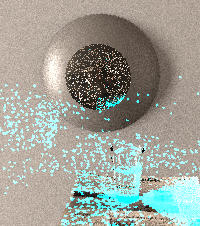
For our caustic photon mapping, photons are emitted from point light sources in the scene, and directed towards the specular object of interest (in our case, the glass of water). The photon map is maintained in a grid data structure, which provides adequate performance for this scene. Because the caustic photons are primarily concentrated in a very small region of the scene, photon mapping adds very little to the rendering time for our image.
Our final image is generated using ~17,000 photons, with radiance estimates obtained for a point by sampling the nearest 20 neighboring photons.
Figure 3: False color visualization of the caustic photon map
The initial performance of our monte carlo area light sampling (from Project 3) was disappointing. We needed to use very high sampling rates to obtain satisfactory image quality, requiring unreasonably long rendering times - a problem that haunted us in the image competition. To improve the sluggish rendering performance, we have subsequently added stratified sampling of the area lights. This yields a reduction in image noise for a given number of samples.
Also, while our original monte carlo implementation sampled area
lights for non-specular surfaces, for specular materials it reverted to
using recursive ray tracing as in the Whitted method. Since the glass
materials in our scene feature multiple specular components (reflectance
and transmission), this recursive trace becomes computationally intensive
when rays are traced deeply. However, such deep tracing of rays is desirable in
our scene - some perceptually significant highlights on the glass of water
are the result of multiple (4 or more) specular scattering events. So, we
modified our monte carlo integrator so that beyond a fixed depth of 3,
subsequent rays are traced stochastically. That is, when more than one
specular component is present, only one is randomly chosen for sampling,
based on their relative weighted contributions to the
ScatteringMixture.
One distressing problem that cropped up when we rendered images at
high rates of supersampling was the appearance of pepper in specular
objects - black pixels where black pixels ought not be. After much
searching, I discovered that in the original lrt
implementation, when a black region of a
PaintedPlasticSurface with roughness 0 is struck exactly
head-on (by a ray in-line with the surface normal to within floating point
precision), the brdf->fr function returns the
Spectrum (nan, nan, nan). This makes its way through the
imaging pipeline, eventually being deposited at an image pixel, which
kills that pixel for good. Oops! Needless to say, this particular
combination of events didn't happen often - and was fun to debug.
We had to add the ability to render a texture map on a heightfield, in order to approximate the newspaper in our real scene. This was fairly straightforward - it required breaking down the u-v parametrization of the heightfield into the appropriate number of subcells for a given grid size. Since there are two triangles per grid square, we break down the the parametrized space appropriately for each triangle.
The second most significant task after photon mapping was to model the brushed metal surface of the clock face itself. This proved harder to get right than expected. In addition to the highlight on the clock from the window to the left (out of shot), there was a lot of diffuse lighting. This made the clock face reasonably well-lit all around. With our sampling methods, we had a hard time recreating these lighting levels.
The model of the surface is basically a regular series of concentric ridges. This is rendered by taking the surface normal at a point and perturbing it perpendicular to the surface's u parameter direction, based on a sinusoidal function of the v parameter. There is a rib file interface consisting of the surface definition "brushedmetal" along with two parameters: "frequency" and "type".
Because our brushed metal surface is disk-shaped, we planned to implement brushed metal for disks and spheres. The "type" parameter allows the RIB file to specify which primitive the surface will be on: "disk" or "sphere". However, the "sphere" parametrization is not fully implemented, and sadly we did not generalize the brushed metal to any arbitrary surface. This should be reasonably easily extended given a way to establish the parametrization direction at a given point (u,v) for an arbitrary primitive.
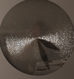
The frequency parameter determines how many cycles or ridges the surface will have as v goes from 0 to 1. Clearly for larger surfaces, larger frequencies should be used to maintain a fine ridge pattern. Typically, frequencies less than 10 or 20 make for easily-visible ridges which do not visually approximate the real appearance of the surface. Frequencies above 40 or 50 are appropriate for showing highlights, but we had difficulty showing both the sharply visible grains and the highlight.
Below is a rendering of our clock with a groove frequency parameter of 10. Notice the moire pattern due to the sampling of this pattern.

This is a rendering of the clock with a higher frequency of grooves. This eliminates the visibility of individual grooves, and makes the highlight more uniform. Notice the bow-tie shape of the highlight resulting from the area light far off to the left of the scene.
Probably the inability of our rendering to really capture the intricacies of the photographed clock face results from a lack of understanding of the complex geometry of the brushed metal surface. Obviously the sinusoidal model is inadequate for capturing the subtleties of the randomness and micro-scale effects of the surface. With a better understanding of the low-level physical realities at the surface of the metal, we would be able to improve our model immensely.