Cloth
Cloth is a very interesting and complicated subject in computer graphics. More accurately referred to as thin-shell material models, the objective is to simulate the motion of thin objects such as cloth, folded paper, clothing, etc. People have come up with a wide array of cloth models, and no single model has proven itself strongly dominant. In order to compare the existing models, we'll break down the model into five categories: equations of motion, integrators, collisions, improvements, and rendering.
Results
A powerpoint presentation corresponding to these topics can be found here.
Various videos of the cloth simulation in action:
Equations of Motion
Mass-Spring Model
The equations of motion for a system govern the motion of the system. One of the first (and simplest) cloth models is as follows: consider the sheet of cloth. Divide it up into a series of approximately evenly spaced masses M. Connect nearby masses by a spring, and use Hooke's Law and Newton's 2nd Law as the equations of motion. Various additions, such as spring damping or angular springs, can be made. A mesh structure proves invaluable for storing the cloth and performing the simulation directly on it. Each vertex can store all of its own local information (velocity, position, forces, etc.) and when it comes time to render, the face information allows for immediate rendering as a normal mesh.
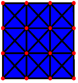
In the cloth structure seen above, the red nodes are vertices, and the black lines are springs. The diagonal springs are necessary to resist collapse of the face; it ensures that the entire cloth does not decompose into a straight line. The blue represents the mesh faces. Looking at the equations of motion:
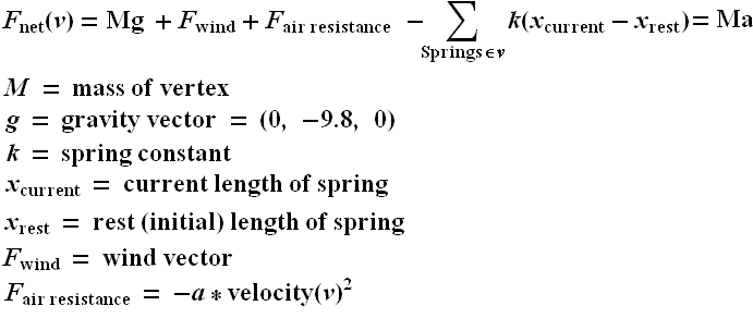
To determine M, a simple constant (say, 1) is fine for all vertices. To be more accurate, you should compute the area of each triangle, and assign 1/3rd of it towards the mass of each incident vertex; this way the mass of the entire cloth is the total area of all the triangles times the mass density of the cloth. The gravity vector can also be an arbitrary vector; if all distance units were meters, time was measured in seconds, and we were on the surface of the earth and "y" was the "up/down" vector, (0, -9.8, 0) would be the correct "g". X(current) is just the current length of the spring, and X(rest), the spring's rest length, needs to be stored in each spring structure. F(wind) can just be some globally varying constant function, say (sin(x*y*t), cos(z*t), sin(cos(5*x*y*z)). a is a simple constant determined by the properties of the surrounding fluid (usually air,) but it can also be used to achieve certain cloth effects, and can help with the numeric stability of the cloth. k is a very important constant; if too low, the cloth will sag unrealistically:
On the other hand, if k is chosen too large, the system will be unrealistically tight (retain its original shape.) Worse yet, the system will be more and more "stiff" the larger k is chosen; this is a mathematical term for explosive. Without careful attention to the integration method, the system will gain energy as a function of time, and the system will explode with vertices tending towards infinity.
Elasticity Model
The mass-spring model above has several shortcommings. Mostly, it is not very physically correct, so attempting to use physically accurate constants is generally unsuccessful. Furthermore it requires guessing arbitrarily which vertices should be connected to which by a spring, and choosing k such that increasing the resolution of the grid leads to a system with similar characteristics can be tricky. A more accurate model, based on integrating an energy over the surface of the cloth, consider energy terms such as:
|
We imagine a giant vector, S, representing every important variable in the system (position and velocities of all the vertices, although potentially there could be more degrees of freedom.) Given energy as a function of the current state of the system, E(S), the equation of motion for a single vertex at position (x, y, z) is then rather simple:
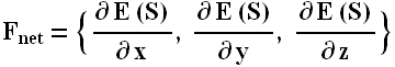
Evaluating this, however, is not so simple. Generally this derivative must be computed analytically. Suppose we attempted to compute the derivative numerically; we consider the state variable constant, reducing our energy E(s) to E(x). We then say:
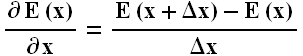
But evaluating the energy E(S) takes a long time; we must iterate over all the vertices, faces, and edges, summing the energy of each one. But we might notice that the effect of x on the energy depends on a very local region (all the incident edges and faces, called the one-ring of the vertex.) So to keep our algorithm O(n) when doing the derivative numerically, we must make sure that we compute E(x) by only considering the energy of the one-ring of the vertex in question.
In general, this method can be very challenging to implement, and although it is physically much more sound, in practice the results are in some ways better and in some ways worse than the mass-spring model. This method of cloth animation, including the derivation of the energy terms, is discussed thoroughly in this paper.
Integrators
After we decide on the cloth model, we need a method to integrate the equation of motion. Assuming our model is newtonian, we have at every vertex defined a position and velocity at each time step t, and our equation of motion tells us dv/dt, or the acceleration of each vertex at time t, and we want to know the position and velocity at the next time step.
Euler's Method (Explicit)
The simplest method for integrating our equations is Euler's method. It goes like this:
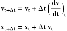
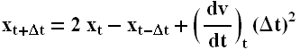
The t subscript on dv/dt means "dv/dt evaluated at time t" (as opposed to say, dv/dt at the previous or the next time step.) Delta t refers to the timestep we're taking (smaller time step means more accurate results but slower computation times.) We can derive the above method quite simply:
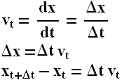
And likewise for the velocity term. This method is very simple to implement, but it has the disadvantage that for most systems, it has a large amount of positive feedback, and tends to cause all variables to rapidly increase to ridiculous values, no matter how small the time step. This explosive behavior is characteristic of all explicit integrators; the term explicit just means that the state at (t+1) is evaluated by just considering the state at time (t). The explosive behavior is arguably the most frustrating aspect of all simulations, and a lot of work goes into dealing with this problem. In cloth, the first way around this is to put enough damping in the system (spring damping, air resistance, velocity damping, etc.) that in a single time step energy decreases the naturally, and the feedback will never occur. Another way is to use one of a vast array of add-ons to the cloth model (discussed later) that prevent the explosive behavior. The only way to solve this problem without altering the model is to use an implicit integrator.
Runge Kutta (Explicit)
Euler's method is not only explosive, it is very inaccurate. As you decrease the time step, the error decreases proportionally. It is possible to use higher-order terms of the derivative to create a much more accurate integrator. There are many such methods, one of the most widely-used of which is called Runge-Kutta. The N-th order Runge-kutta algorithm considers derivative terms up to the N-th order. For various reasons, 4th order is considered optimal, since it gurantees the integrator error decreases proportional to the fourth power of the time step (and it is not true that 5-th order is proportional to the fifth power of the time step.) The algorithm is also excellent because it still only needs the first derivative; higher derivatives are efficently computed numerically just by knowing how to compute the first derivative. While very accurate, it takes slightly longer to compute, and still suffers from all the problems of explicit models, so even if it takes the system longer to explode, in general it still will.
Verlet Algorithm (Explicit)
The Verlet integration algorithm is such an explicit model with the very interesting propety that it does not need to know anything about the velocity; it computes this internally via looking at the position at both the current and previous time step.
Another wonderful aspect of this algorithm is that like 4th order Runge-Kutta, it is 4th order accurate. Because it is quite accurate, easy to implement, and does not need the velocity terms, it is my favorite explicit model and the one I use in all my cloth models.
Euler's Method (Implicit)
Unlike an explicit integrator, an implicit integrator uses the state variable at the current time step and the derivative at the next time step to compute the state variable at the next time step. There is a perfect implicit analogy to Euler's method; in our model, we have the following equations:
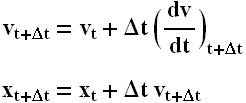
The only change is the subscript from "t" to "t + dt". We notice quickly that we only need to deal with the v(t+1) term; the x(t+1) term can then be trivially computed using this new velocity. But computing this new velocity can be extremely tricky. In either the mass-spring or elasticity model, this requires the following: consider the big state vector S (all the velocities and positions in the system) as a 6n x 1 matrix (where n is the number of vertices. Linearize the equations of motion so we can represent dv/dt at time t as follows:
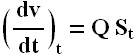
Where Q is a giant 3n by 6n matrix representing the linear relationship between the change in velocities and the state of the system. We would then substitute this into the implicit euler equation for dv/dt, and solve for the velocity at the new time step. However, this would involve inverting the massive matrix Q (which is thankfully very sparse, assuming not every vertex is connected to every other vertex.) This is generally accomplished with linear conjugate gradient descent. If you're interested in implementing this, see this paper (the same paper as above.) Overall, this algorithm is very complicated to implement for cloth models, but because of the negative feedback, the energy in the system tends to decrease, rather than increase explosively. This enables you to take much larger time steps and remain stable, and avoids the necessity of excessive damping terms. However, it is very time consuming to take each time step, requires convergence of a matrix inversion algorithm, and because such large time steps are taken and the relationship between error and time step is linear (as with Explicit Euler's,) the algorithm is a very bad approximation of the underlying motion we are integrating.
Higher order implicit algorithms
One might expect that there is an implicit analogy to Runge-Kutta. While such an analogy exists, and has both the advantage of good errors and a stable system, I have never seen it applied to cloth models; the 1st-order implicit version is sufficently complicated for anyone.
Symplectic Euler's Method (Semi-Implicit)
Many algorithms exist which are compromises between implicit and explicit models. A simple one is called Symplectic Euler's Method. It's equation of motion is:
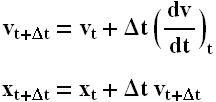
It is called semi-implicit because it computes the velocity explicitly, but the new position implicitly. This helps reduce the feedback (positive or negative) and can greatly improve stability, at no cost in algorithmic complexity. It also has the powerful advantage that in many systems it conserves energy on average. However, it does not conserve phase or oscillatory motion: in cloth, this results in strange out-of-phase circulations occurring all over the mesh, so in general this algorithm is not a good choice for cloth. Higher order symplectic models exist, but they have similar properties, except for the higher order accuracy.
Collisions
There is no avoiding it; collisions are very hard to deal with when it comes to cloth. Doing it in a physically accurate manner is a complete nightmare, and I have never read a paper that claims to have implemented this. Hacking up a solution with even reasonably plausible results is challenging enough; making gurantees about the cloth not interescting itself or not intersecting other objects is also challenging, but some papers propose complicated models that claim to have this propety; certainly, they have very visually pleasing results. To approach the collision problem, we break it down into two types: cloth-cloth, and cloth-object.
Cloth-Object Collisions
Generally the easier of the two types of collisions to deal with, we assume we have some solid objects in the scene, and independent of their motion, their position at and around time t is fixed and known. These objects might be represented as geometric primitives (cylinders, spheres, cubes, etc.) or the interior of a mesh.
Physically Correct Model
The physically correct method of cloth-object collisions is as follows:
|
This algorithm is extremely annoying to implement and slow, because we will end up creeping along very slowly as we have to keep stepping forward, noticing a collision, backing up, and repeating. Adaptive time stepping doesn't even help, since we have no choice but to make small time steps all the time. While some papers claim to deal with the friction forces correctly, almost all of them refuse to back the system up, instead making some best guess as to the correct location of the face.
Easy-to-implement Model
In practice the above is very annoying; even detecting the collision can be frustrating since the path taken inbetween the two time steps is a prism-like volume. The model I use is considerably more problematic but reasonable to implement. Firstly, we do not deal with faces or edges at all, and we do not deal with the intermediate time steps; any of the cases below will be missed by my algorithm (red = initial position, blue = new position.)
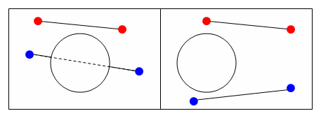
The only thing my algorithm considers is if a vertex at the positions computed for the next time step is inside one of the objects in the scene, we detect a collision. Our response can be one of two things: move the vertex back to where it came from (this is equivalent to an infinite-friction surface) or we could "repel" the object in some fashion. Given a position, many objects have a natural point on the surface associated with it. Take for example a sphere; given a position, consider the intersection of the sphere with the line from the sphere's center to this position. This point is the closest point on the surface associated with the input point, and while such a position is well defined for all objects, it is especially easy to compute in the case of simple geometric objects. If, rather than moving a point back to its original location we move it to its "repelled" point, we will give the visual apperance of a very slippery (almost zero friction) surface. In the limit as our cloth is refined, with more and more vertices and smaller and smaller faces, the fact that we consider only vertices will be irrelivant, and this model will perform reasonably well.
|
|---|
| A cloth held at two corners resting on a sphere |
Cloth-Cloth Collisions
Cloth looks very unrealistic if it passes through itself. A simple solution is as follows: if two regions of the cloth are too close to each other, apply a repulsive force to the vertices around this region, encouraging seperation. This is very ugly, in practice, since it is very sensitive to the definition of "too close", the choice of time step, the choice of the repulsive forces, and can further contribute to numeric instability. Despite all of these problems, it is what this paper does. I don't like this method and have never implemented it.
A seperate, powerful solution is as follows: compute the new positions and determine any intersections that happened. Now go back to the previous time step, and modify the magnitudes of the velocities in such a way that the collisions no longer occur. This is both not too hard to implement, effective in practice, and can gurantee that no collisions occur. However, determining all the collisions is very time consuming and greatly slows down the algorithm, in addition to causing a geometric headache. So the algorithm I use is different from both of these approaches.
My algorithm considers the cloth as a set of connected marbles. We imagine a virtual marble to be centered around each vertex. Marbles are not considered to be touching if their associated vertices are connected by a spring; thus, we can set the radius of a marble larger than the distance between two vertices. If we do this, then we have covered the entire surface of the cloth, and if no two marbles pass through each other between t and t + dt, the cloth has not intersected itself. The update algorithm is very simple: if the new positions contain vertices whose marbles are inside each other (the distance between the vertices is less than twice the marble radius,) back the vertices up such that this collision has no occured (although we remain at the new time step.) We can make several choices about the velocities; generally it is simplest to zero the new velocities, although it is possible to get "bouncing off" effects if desired. In general this algorithm works well and in my opinion is the easiest to implement.
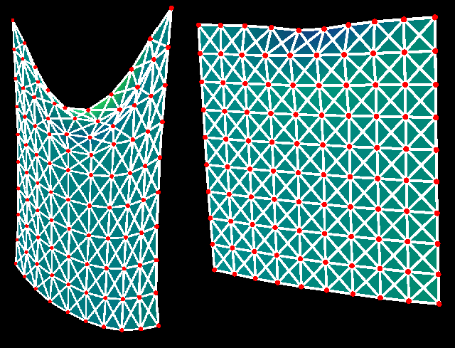
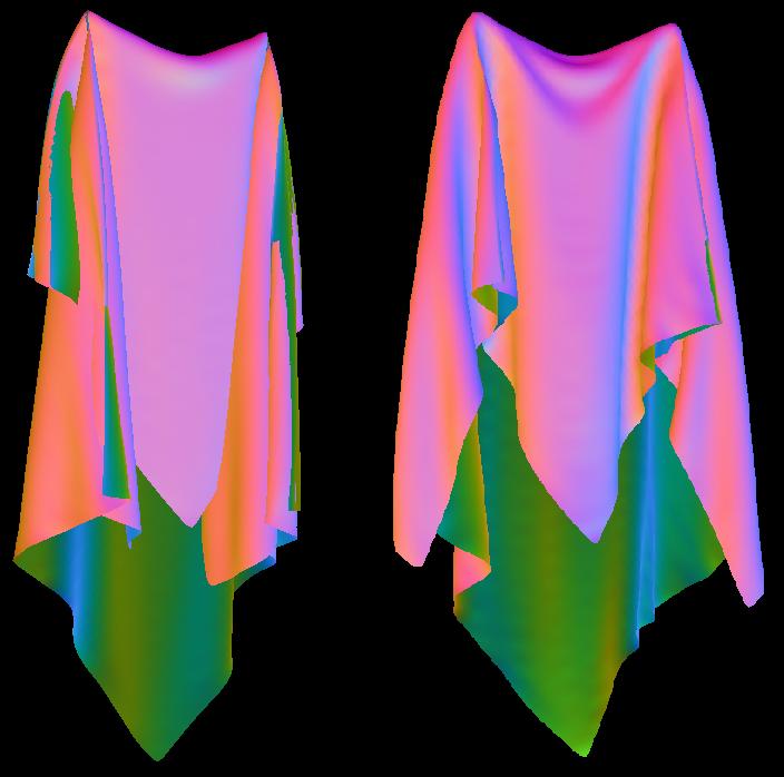
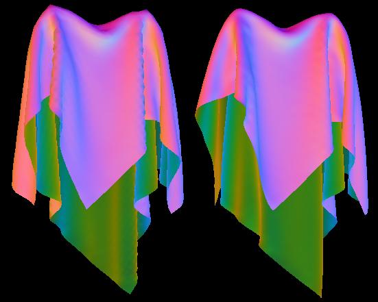
Suppose we start with a planar cloth and fix two arbitrary vertices in the middle of the cloth. Without cloth-cloth collisions, the cloth will settle into a position where it is highly self-intsersecting, but with the cloth-cloth collision algorithm above we avoid this interpenetration and get very convincing cloth-like folds.
|
|---|
| Left: no cloth-cloth collisions, Right: cloth-cloth collisions active |
Improvements
Maximum Stretch
The idea of maximum stretch is the savior of all exploding cloth simulations. The idea is very simple: whenever two connected vertices are stretched beyond a certain maximum ratio compared to their rest distance (say 110%, so 10% stretch) move them such that they are stretched at exactly 10%. Likewise we can say that whenever two connected vertices are compressed closer than 90%, place them at exactly 90% compression. We do not bother backing the simulation up once we hit one of these, but rather after updating all the positions we iterate through all edges, compressing or stretching the attached vertices as necessary each time to keep them within the 90% to 110% of their rest length. Of course, moving later edges may cause previous edges to violate their stretch conditions, so we need to iterate through many times. But even if we do not entirely satisify the condition for every edge, our overall goal is accomplished: the energy of the system will not explode, and the cloth will always settle into a reasonable configuration. The huge advantage of this is that we can use an explicit integrator (such as Verlet) without incredibly small time steps. Another benefit is that we can avoid the cloth sagging unrealistically even with a low k, because the maximum stretch being 10% acts as an infinite k for high stretch and a low k for low stretch. This is also rather realisitc: cloth, in general, is easy to stretch for small displacements, and becomes very tough once its fibers reach a certain tension. Finally, using an explicit model will generally gurantee that a change at node A cannot affect the motion at node B, N edges away, until at least N frames later. With this edge constraint mechanism, extreme motion at A can affect the entire cloth in a single frame, a very useful feature if you attempt to move the cloth vertices around very rapidly.
Bending Springs
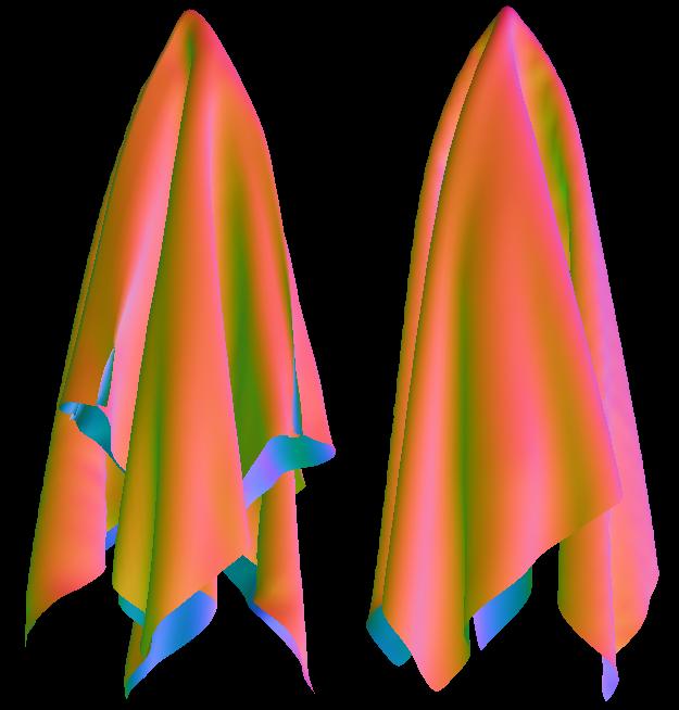
Rather than just connecting a vertex to its immediate neighboors by a spring, we can attach a vertex to its more distant, "two-ring" neighboors, as well. The strength of these long-range springs compared to the base strength can be thought of as a bending strength, since resistance to this kind of motion will keep the cloth locally more flat. This is especially useful to remove local wrinkling of the surface when the resolution of the cloth is very fine.
|
|---|
| Left: no bending springs, right: bending springs with high k |
Rendering
Subdivision
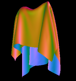
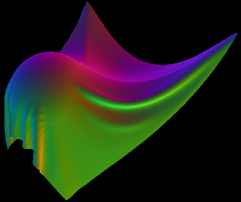
The cloth structure can be easily rendered by using the triangle structure of the original mesh. I tend to use a rather odd normal xyz to vertex RGB coloring scheme, because it makes it ovbious what the orientation of the cloth at any point is (and hence any inter-penetration is immediately noticed.) However, no matter what color scheme is used, it is nice to have a very smooth piece of cloth, without the need for millions of simulation vertices. Subdivisional surfaces is a very powerful algorithm to accomplish this; we can take a low-resolution cloth simulation output, and construct a high-resolution refined mesh. The result is only as accurate as the initial resolution, but the result is always a smooth surface. In the case below, I use the loop subdivision scheme.
|
|---|
| 20x20 grid with two fixed vertices. Left = No subdivision, Mid = 1 level of subdivision, Right = 2 levels of subdivision |
We can see that even on a coarse grid, one level of subdivision makes the image incredibly smooth. Repeating the simulation on a 50x50 grid, again we see subdivision removing many nasty rendering artifacts.
|
|---|
| 50x50 grid with two fixed vertices. Left = No subdivision, Right = 1 level of subdivision |
Quilting
With or without subdivision, our cloth still looks like an infinitely thin piece of paper. However many types of thin shells have a very visible thickness, such as a quilt or cotton sweater. Rather than simulating a thick piece of cloth, what we want is to take our infinitely thin output of the simulator and construct a mesh with thickness from it. Such an algorithm is relatively straightforward, given the right machinery. We first define a function f(x, y, z):
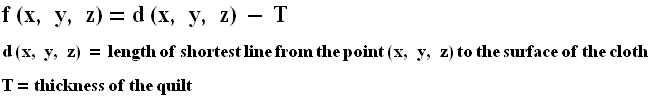
The surface f(x, y, z) = 0 is then "the set of all points a distance exactly T from the surface of the cloth." Once we can compute this function for any (x, y, z,) we want an algorithm that will give a triangular approximation of this surface and we are done. An algorithm that accomplishes this is called marching cubes, which divides the world we're trying to pologonize into a set of evenly spaced cubes, samples the function f(x, y, z) at each corner, and for cubes with some vertices with f(x, y, z) > 0 and some vertices with f(x, y, z) < 0, constructs a triangular approximation of the interior.
|
|---|
| Left: Thin cloth input, Right: marching cubes output |
Zooming in and looking at the wireframe:
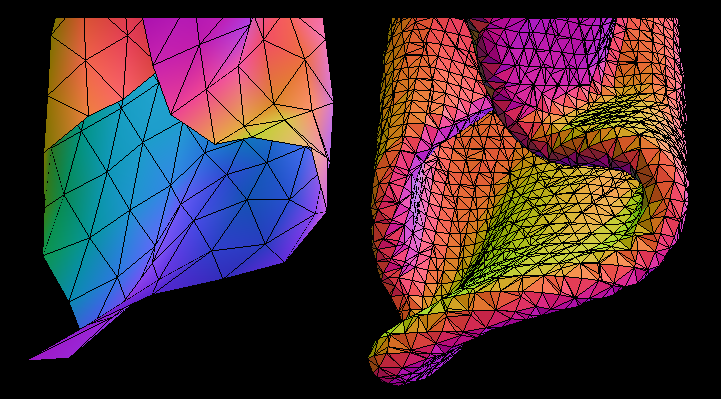
|
|---|
| Left: Thin cloth input, Right: marching cubes output |
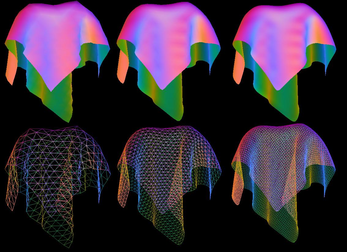
By increasing the resolution of the marching cubes, we can make the approximation as close as we wish. However, marching cubes does not give us a very uniform triangulation of the surface, and this is very problematic when we try to compute normals or render, as many triangles have almost zero area. To solve this, we first simplify the mesh producing many less vertices, and then we perform subdivision on the resulting mesh, finally refitting it to the original surface f(x, y, z). Both of these steps have a lot of work supporting them, but they are very well defined operations. Personally, I use my own subdivision code but invoke DirectX code to simplify the mesh to a desired number of faces/vertices. The results, shown below, is a very nice quilted mesh.
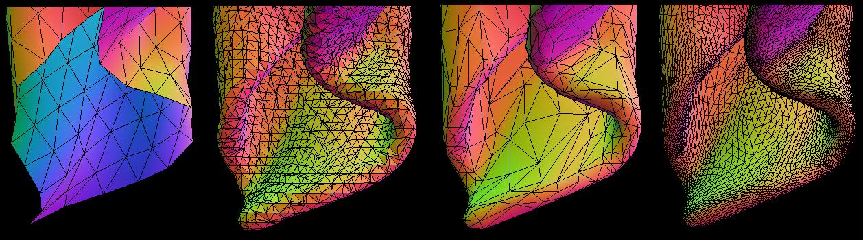
|
|---|
| From left to right: Initial flat mesh, marching cubes approximation, simplified mesh, subdivision of simplified mesh |
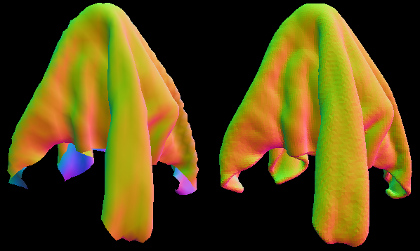
We can do many other tricks using this quilting; for example, if we define d(x, y, z) as the distance to a vertex on the initial cloth, rather than the distance to the surface of the cloth, we will get a "knot" at each source vertex. This can make for an interesting surface pattern, shown below, and many more can be achieved by allowing thickness to vary (and go to zero) across the cloth surface, creating holes and clumps derived from an input texture.
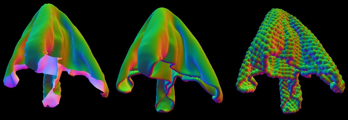
|
|---|
| From left to right: Initial flat mesh, quilt with f(x, y, z) as distance to surface, quilt with f(x, y, z) as distance to vertex |