An Autostereoscopic Display for Light Fields
http://graphics.stanford.edu/~billyc/research/autostereo
|
|
SUMMARY
An autostereoscopic display shows an image to a viewer without any use of googles or other devices. The image is appealing because it follows many of the principals of 3D objects in the real world. [5] This viewing model has been around since the turn of the 20th century and has been as popular as 3D movies or holograms. The key contribution is the ability for the viewer to see parallax in an image as he changes his viewing position -- yielding the effect of 3D.
Recently in 1996, the introduction of light field/lumigraph rendering allowed viewers to examine a 3D model or scene independent of scene complexity. Additionally, the sampled 2D image could be constructed from light rays measured from real irradiance from the scene to the camera's image plane, giving the viewer a highly realistic (synthetic) image of the model or scene. While such convincing images can be rendered, one limitation is the two-dimensionality of the display device.
To date, few researchers have explored the possibilties with viewing a light field on an autostereoscopic display; the notable exception being McMillan and his colleagues at MIT who demonstrated how to construct and print an image for use in combination with a hex lens-sheet to achieve an autostereoscopic image of a light field. [16]
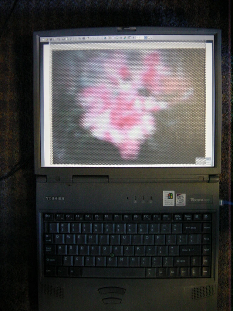
I propose to extend the work of McMillan et al. and build an autostereoscopic display where instead of a printed image, I use the display-monitor -- trading spatial resolution for dynamic light-field sampling. Where the MIT group create an autostereoscopic image for a static lightfield, a display can handle dynamic light fields, such as those produced by the Stanford Light Field Camera Array. Additionally, other than the lens sheet, no extra hardware is needed to view dynamic light fields since the lens attaches to the display device.
Because anyone can obtain the necessary lens-sheet, it becomes feasible for anyone and everyone to obtain autostereoscopic displays for their home. A subgoal is to write the necessary drivers to convert a conventional display into an autostereoscopic device (to use, for example in 3D Desktops).
HARDWARE
- Big Bertha (IBM T220) (211 2/3 pixels/inch) (.12mm pixel spacing)
- Dell Inspiron 8000 Laptop (12'x9') (1400x1050 pixels) (116 2/3 pixels/inch) (13611 sq pixels/sq inch)
- Hex Array (Conventional Lens [Fresnel #300]) (.09 in) (101.57 sq pixels / lenslet -- for laptop)
CALIBRATION
For a given lenslet, we want to compute a mapping from angle to pixel. Suppose we construct a parameterization as shown in Figure 1. The constants are taken from the Frenel Lenses lens catalog for hexagonal array #300. Ci are the centers (optical centers) of the lenslets, the bold arc of the circle represents the visable refractive surface (facing upwards). Fi are the focal points of the i'th lens. The lenslets (measured from their centers Ci) are placed 0.09 inches apart (lenslets along the orthogonal direction are placed 0.18 inches apart due to the hexagonal pattern of the lenslet array). The thickness of the lenslet array is measured from the center of the lenslet. In this case, the thickness is 0.12 in. which is donoted by the horizonal line at z=0.165 in.
 Figure 1. A parameterization of a lenslet.
Finding the maximum FOV
Given this parameterization, it's
useful to find the maximum field of view for any given lenslet. This will
also tell us what the pixel coverage is of a given lenslet. The red line
PT1 is a ray of light. The blue line PF1 is the pixel coverage we want to
determine -- assuming that the pixels are flush with the back of the
lenslet array.
Note that |C1C2| and |T1C2| are known. Where |x| denote magnitude of x. Then Θ = arcsin(0.045/0.09) = 30°. Hence, the FOV = 180-2Θ = 120°.
Similarly, |PF1| = |C1F1|/tan(30°) = 0.2078 in. The lenslet diameter is .09 in., so the pixel coverage at maximum FOV actually overlaps with several pixels over adjacent lenslets. In fact, there is a 0.1628 in. ((2*0.2078-0.09)/2) overlap if the maximum FOV is used.
Finding the maximum constrained FOV
Given that the maximum FOV causes overlap, I want to find the maximum FOV
which does not have pixel overlap, which I call the maximum constrained
FOV. The green line P2T2 is a good candidate for the maximum constrained
FOV. In fact, it can be proved that P2T2 denotes the widest angle ray if
we assume a paraxial lens approximation.
If the green line P2T2 forms the angle of maximum constrained FOV (measured with respect to the paraxial ray of the lenslet), then any other line forming a larger FOV must overlap adjacent pixel areas. Let's pick any ray forming a larger FOV, then its point of intersection on the focal plane must coincide with a parallel ray that intersects the optical center. In the case of a spherical lens, this ray can be found by finding the pt on the sphere where the ray is normal to the sphere surface. Obviously, this point must be to the right of T2, since the ray forms a greater angle to the surface pt at T2 (since it has a larger FOV). Since this intersection point is to the right of T2, and its ray intersects the optical center, then the intersection of this ray and the focal plane must lie to the left of P2. But P2 is the leftmost pixel under the orthogonal projection of the diameter of the lenslet, so the new intersection must lie in a neighboring pixel area. Hence, any ray creating a larger FOV than the FOV formed by P2T2 will be in neighboring pixel areas, so P2T2 forms the maximum constrained FOV.
The maximum constrained FOV = 2*atan(r/f) = 2*atan(.045/.12) = 41.11° where r is the radius of a lenslet, and f is its focal length.
Another approach that uses empirical data is to use the Faro arm with a camera attached to view a calibration image.
CREATING AN AUTOSTEREOSCOPIC IMAGE
Once a mapping is found between angles and pixels, an image must be produced to reflect that mapping. Figure 2 shows a generic configuration for an autostereoscopic image.
Figure 2. Some intuition on how the autostereoscopic image should be produced. Image used with permission from Paul Bourke [6].
In the case of light fields, each subimage used for compositing is a 2D
slice of the 4D field, where the slices are obtained from placing a
virtual camera at the optical center of each lenslet. See Figure 3.
Figure 3. Sampling the 4D light field
RELATED PAPERS
Holography, Stereograms, Autostereoscopic Displays- ACM Siggraph 89 Course Notes
- Ames, A. Jr., "The Illusion of depth from single pictures", J. Opt. Soc. Am., V10, pp137, 1925.
- Benton, Stephen A. "Display Holography: an SPIE Critical Review of Technology" Proc. SPIE, Holography, A86-32351 14-35, (1985), pp. 8-13.
- Benton, Stephen A. "Survey of Holographic Stereograms". Proc. SPIE, Processing and Display of Three-Dimensional Data, 367, (1982), pp. 15-19.
- Halle, Michael, "Autostereoscopic Displays and Computer Graphics", Computer Graphics Volume 31, Number 2, May 1997.
- http://astronomy.swin.edu.au/~pbourke/stereographics/lenticular/
- Ives, H. E., "A Camera for making Parallax Panoramagrams", J. Opt. Soc. Amer. 17, pp435-439, Dec 1928.
- Lucente, Mark and Tinsley A. Galyean. "Rendering Interactive Holographic Images", Proceedings of SIGGRAPH '95 (Los Angeles, CA, Aug. 6-11, 1995).
- Okoshi, T., "Three Dimensional Imaging Techniques", Academic Press, New York, 1976.
- McAllister, D. F., Robbins, W. E., "Progress in projection of parallax-panoramagrams onto wide-angle lenticular screens", SPIE 761, pp35-43, 1987.
- Robbins, W. E., "Computer Generated Lenticular Stereograms", Proc. SPIE 1083, 1989.
- Sandin, Daniel J., et al., "Computer Generated Barrier Strip Autostereography", Proc SPIE, Non-Holographic True 3D Display Technologies, 1083 Jan 1989, pp65.
- Saxby, Graham. "Practical Holography", 2nd edition. Prentice Hall, Dec. 1994.
- Stevens, R. F., Davies N., "Lens arrays and photography", Journal of Photographic Science, 39(5):199-208,1991.
- Gortler, Steven J., Grzeszczuk, Radek, Szeliski, Richard, Cohen, Michael F., "The lumigraph", SIGGRAPH 96, pages 43 54, 1996.
- Isaksen, A., McMillan, L., Gortler, S.J., Dynamically reparameterized light fields, Proc. Siggraph 2000
- Levoy, Marc, Hanrahan, Pat, "Light field rendering", SIGGRAPH 96, pages 31 42, 1996.