IMPLEMENTED ALGORITHM
Our segmentation and tracking algorithm can be separated according to this
flowchart:
The segmentation is the top box, and the tracking is the bottom box.
Image Segmentation
The finalized segmentation process undergoes 3 processes:
- skin detection
- background removal
- general Gaussian and morphology filters
During skin detection, an initial silhouette is manually traced over the diver's initial pose. Those pixel values inside the silhouette are used to compute the mean HSV value of the skin.
A manual silhouette for the image sequences generated for kurt1
Using this mean value for skin pixels, we iterate over all pixels in the image and remove any pixels whose values are greater than a given deviation:
One frame where "non-skin" pixels have been removed. Notice that the
pool is mainly gone. But closer pixel values such as the fence remain.
However, this method proved insufficient since most of the background remained. Next we used a simple background subtraction algorithm which takes the last n frames of the video and computes an average per pixel.
Let S(x,y) be the sum of pixels (over n frames), and Sq(x,y) be their
squares. Then at each x,y location, m(x,y) = S(x,y)/n and the standard
deviation is sigma(x,y) = sqrt(Sq(x,y)/n - (S(x,y)/n)^2).

If a pixel at x,y satisfies the condition: abs(m(x,y) - p(x,y) >
3sigma(x,y) then it's considered part of the foreground. [OpenCV pg32]
These averages are compared to the frame in question and if this difference is greater than some deviation then that pixel is considered a foreground pixel. Note: We decided not to use the bayesian skin classifier because we wanted to see if a simpler method existed and we did not want to force a restriction of having a training set.
Values after background subtraction. Due to unstable camera photage,
the fence still remains because of deviations in pixel locations. A
Gaussian was also applied.
Since much of the image has noise (ie: the fence in the figure above), we can apply certain morphology filters (erode) to help remove such noise. A morphology filter uses an image A and and a structuring element B (aka kernel). The filter was originally used for set operations.
If we let B_t be the translation of B around the image, then the dialate
of A by B is:
Similarly, the erosion of an image A is given by:
Basically, the dilate filter "grows" pixels around existing pixels and the erode filter trims the edges.
Illustration of Dilating and Eroding
Diagrams and equations taken from OpenCV Manual pg75.
After applying a 5x5 Gaussian and the erode morphology filter.
However, there still is a lot of noise after the erosion, so we tried applying a locality filter where hypothesized silhouette values are "local" to the previous silhouette, but this turned out disastrous since the locality constraint couldn't keep up with the moving diver. See Bloopers.
Tracking
Our goal for tracking was to track the diver after segmentation -- with
the intention of having segmentation give tracking an easier job. Our
first tracker implemented a pyramidal Lucas-Kanade optical flow, but that
turned out disastrous. See Bloopers.
So instead we used a ConDensation tracker that simply tracked the centroid
of the skin-colored pixels. The center of the window corresponds to the
centroid. In most of our footage, our tracker seemed to follow the diver
pretty well.
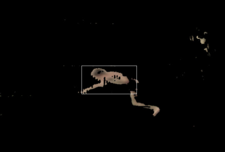
Tracking window on a single frame
We used the window as a mask to zero out all the pixels outside the
window.
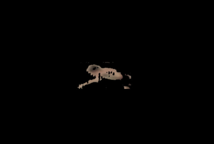
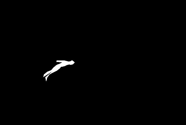
After using the tracking window as a mask
Disparity Calculation
Global Vector Disparity Calculation via Motion History Images. Once
silhouettes have been extracted per image, one can composite them into a
single image where the intensity of each successive silhouette is maximum,
and the previous silhouettes decrease in intensity, effectively yielding
an image like:
A MHI of 10 frames. The multiple rectangles are from the Condensation
tracker. The dots are due to segmentation limitations, but removed later
on by the tracker
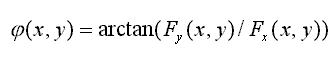
We then convolve the MHI image with two separable PreWitt kernels to extract the X and Y magnitudes of the gradient vector. Then the orientation is simply:
Note that since intensity values on the silhouette image are discrete, all non-zero gradients are clustered around the "steps" and edges against the background. However, the gradient at a particular point is meaningful only when it lies on the step, and therefore, we must zero out all the vectors adjacent to the background pixels (i.e: black) before computing the global vector. A global vector is simply an aggregate of all the gradients, normalized by the total number of valid points. It signifies the general direction of the blob. By successively adding the global vectors over the time starting to absolute coordinate (0,0), we can derive an approxipate trajectory in 2D space.

A segment of the motion history image (magnified by 3X).

Before discarding unmeaningful gradients on the edges
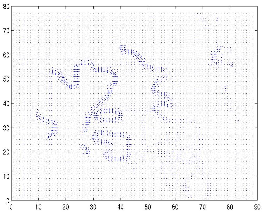
After discarding unmeaningful gradients on the edges
Another way of determining the general direction of the blob is by computing the centroids of the blob in question. Once again, motion history images are used because the successive layers of the past tend to stabilize the movement of the centroids over time. More weight is given to the more recent layer.
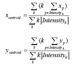
Both methods are highly sensitive to garbage left over by the segmentation process. Fortunately, the condensation tracking filter, which defines a rectangular region of interest and zeros out pixel values outside of the region, improves the accuracy of the centroid computation significantly.
Each of the above two methods returns a set of (x_i,y_i) coordinates, which may be used to fit a polynomial function. Since the camera is stationary and that the diver must obey the law of gravity, the trajectory should essentially resemble the shape of a paranola. However, we discovered that a simple quadratic function did not fit well due to photages containing scenes beyond the window of the actual dive, such as divers submerged under water, or ducking on the platform prior to jumping into the air. Instead of a second-degree polynomal function, we decided to fit a third-degree polynomal function using the least square solution to allow a certain degree of flexibility.
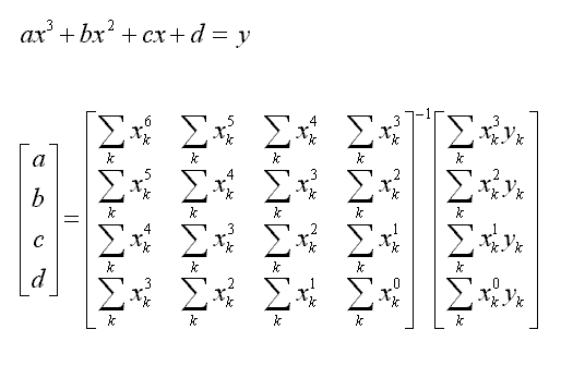
One advantage of using trajectory curves as the basis of comparison is that their characterizations are invariant to the rate of video sampling. We don't have to worry about comparing a sequence played back at normal speed with another shown in slow motion. Another advantage is that it models a physical constraint, the law of gravity, conveniently. This constaint restricts the form of the curve function so it's not completely arbitrary. Finally, a prior knowledge like newtonian mechanics could be used to predict the centroid location in the next frame. I imagine this could be useful to further improve the performance of the tracker.
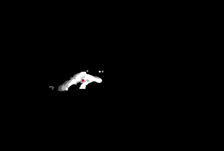
The red dot is the computed centroid for this particular image.
Note that the accuracy of the centroid estimation improved
dramatically after the condensation tracking filter.
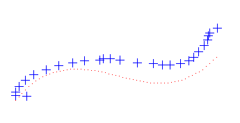
The blue markers represent an instance of the (x_i,y_i) coordinates (x
and y axies not shown in figure). The dotted red line represents the
best-fitting third-degree polynomial function. In case you haven't
noticed, this is Vaihbov ducking slightly at the edge of the pool before
jumping into air executing a beautiful dive.
After fitting polynomial curves onto the trajectories, we simply computed the affine mapping from one curve to another. We ignored translation and rotation, so all we were left with was scaling in the x- and y-directions. If the two divers were perfectly synchronized, this matrix would be the identity. So, we compared the affine mapping to the identity to arrive at a disparity measure. We penalized equally for differences of scale in x and y, but perhaps if we knew more about diving then we'd penalize more for one than the other.
Planar Tracking (cardboard people)
You might say a good synchronized dive requires more than just a good
parabolic match. Simply deriving the trajectory based on centroids or
global vectors hardly exploits the wealth of information encoded
in a diving sequence, such as bodily configuration. Parameterizing a
full human body (i.e: skeleton and flesh) in a full 3D space is
obviously not feasible for this project, but given the numerous
constraints in our water diving environment, we can apply several
simplification steps that do not overly compromise the worthiness of
the model.
Constraints:
- Lateral view from a stationary camera. This eliminates the need for parameterizing the camera configuration, and there is no relevant information lost due to occlusion.
- No twist or fancy dive; just straight dive or somersault. Combined with that lateral view constraint, we can approximate the diver configuration with a flat model instead of a full blown 3D one. Big saving in implementation effort, computation cost, and potential debugging nightmare.
- Physical constaints with the human body. Joints do not usually separate, and bones do not usually bend, and there are only so many segments seen laterally.
Simplifications:
- We used three body segments: one for torso, two for the two sections of legs. It's true that we could've added one more segment representing the diver's arms, but that was decidedly too costly.
- Each of the three segments may be oriented at any angle, ranging from 0 to 360 degrees. We will not prohibit certain impossible human configuration (e.g: knee touching the back of your head) to simplify the search routine.
- Fixed segment length and width, and absolutely no deformation allowed. Too troublesome to implement.
Therefore, our internal model is in a 7-dimensional space:
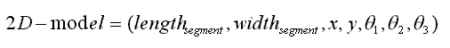
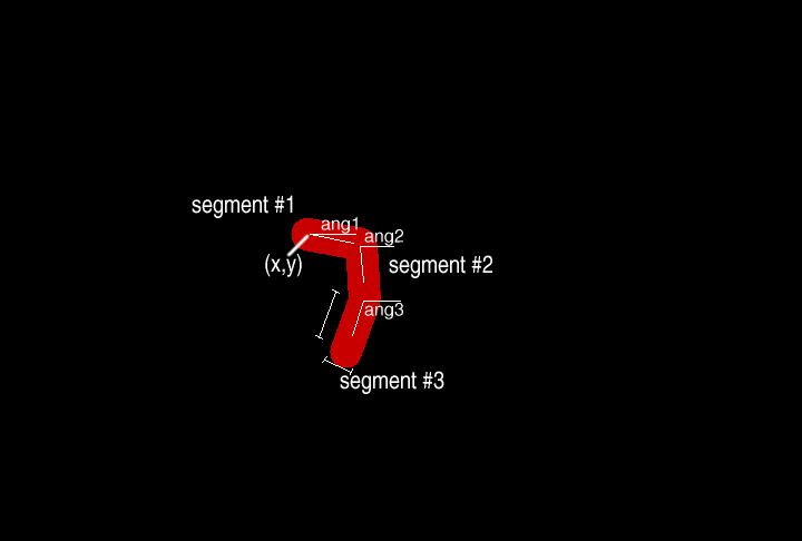
A projection of the internal model.
The tracking begins with a manual initialization of the model matching the first frame of the photage. Automating this would probably be difficult, so we did not attempt.
At every frame, we have to somehow adjust the parameters of the model that should best fit the diver on the next frame. The search of the configuration space follows this form:
- loop N times
- adjust each parameter slightly by a small constant amount (delta values), individually and non-cumulatively. Remember the one that minimizes the error function.
- commit this one parameter change
Ideally, we want to be able to traverse the entire space of configuration to find the globally optimal point, but that's obviously too expensive. An alternative is to search around the immediate neighbors, but that also is very expensive because in a 7D-space, there are 14 possible individual adjustments, and testing all immediate neighbors require 2^14 combinations (i.e: power set).
Instead, we will adjust one parameter at a time, and allow N iterations in the hope that the search algorithm will locate the local minimum (error). In a way, this models the physical constraint where body parts may be not move across the 2D space too much in a certain amount of time, such as time elasped between each consecutive frames. Note that not testing all immediate neighbors might not lead to a locally minimum because of possible "ridges" in the search space. This is the price we pay for the simplification.
We found that (N=10, translational_delta=4pixels, and angular_delta=4degrees) was effective while keeping the computation cost acceptable.
The difference function is defined simply as:
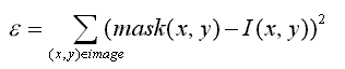
The projection of our internal model (red) superimposed onto an intensity map.
Using an correspondence algorithm such as this frequently leads to an irrecoverable divergence. It's particularly distastrous if there are a lot of garbage left over from the segmentation stage. Fortunately, the condensation tracker at least discards the junk outside of the window, so the risk of the model leaving the intended region is minimized. Furthermore, the successive layers of the motion history image help pin down the model to the right place.
The output of the cardboard tracker is a sequence of model configurations. Much more information about the diving performance is extracted this way compared to the simple center of mass trajectory. Complex characterizations of a dive, such as somersaults and torso orientation, can be easily derived from this model. However, this tracker is much more susceptible to mistracking due to divergence, and it's highly computationally expensive.