Subdivision
Subdivision is a powerful and easily implemented algorithm used, in its simplest application, to smooth meshes. The underlying concepts are derived from spline refinement algorithms, but the idea is that there exists a well-defined smooth surface associated with any given input mesh (the exact surface depends on the subdivision algorithm used.) We define a refinement operation, that takes the input mesh and generates an output mesh that is closer to the surface. If we apply this refinement process infinitely, we will exactly achieve the target surface. However, after just a few levels of refinement, we are generally close enough to the limit surface that they are visually indistinguishable. Depending on the type of input mesh (triangular, quadrilateral, etc.) we must use a different subdivision algorithm, and within triangular meshes there are still a wide array, although some are visually superior to others. Quadrilateral based meshes generally use Catmull-Clark, while triangular based meshes generally use loop subdivision.
Loop Subdivision
All subdivision algorithms start by replacing the geometric element (in our case, a triangle) with smaller versions of the same element. In the 3D case of tetrahedrons, this is very complicated, but in the case of triangles it is trivial:
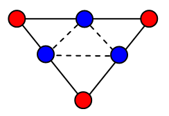
For every edge in the source mesh, add a vertex (shown in blue,) and for every triangle on the mesh, create the four triangles shown above. The exact geometric location of these new edge vertices, and the new coordinates of the intial vertices, are all determined by the subdivision scheme. In every case, however, they are linear combinations of the source mesh vertices, and the source mesh vertices that contribute to a point's new location are only a few edge or triangle hops away. The edge vertices are the easiest to deal with:
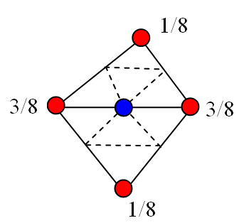
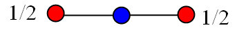
Every edge in the source mesh has two adjacent faces (we'll deal with boundaries later,) and from these we can find the two "opposite" vertices. Of course each edge also has two connected vertices, and we just take the a linear combination of the source vertices in the ratios shown above, and we have the location of the vertex associated with this edge.
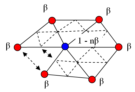
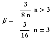
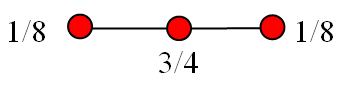
Every vertex in the source mesh is also in the subdivided mesh. Its new position is computed above, and depends on all the vertices connected to the vertex by an edge. The number of such vertices, n, determines the constant beta. There are many options avaliable, but the simplest choice is
The boundary cases are based off basic spline refinement schemes and are equally simple. For a new edge vertex:
And for a boundary vertex:
|
|---|
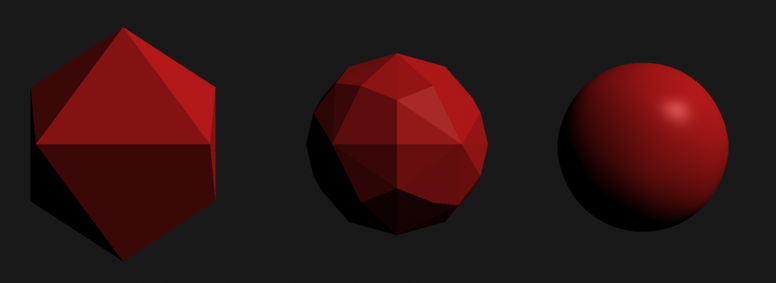
| Catmull Clark subdivision on an icosahedron. The right-most mesh is the result of several iterations. |
|
|---|
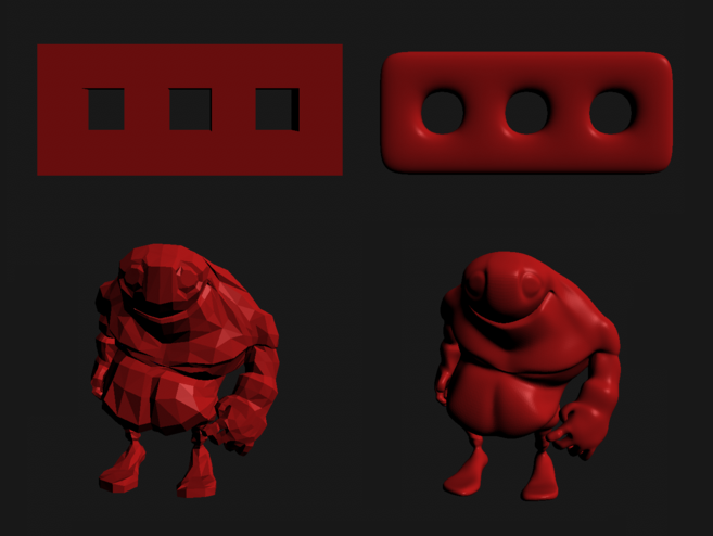
| Catmull Clark subdivision on a 3-holed torus and a character. |
You can find an explination of Catmull-Clark subdivision here.