The previous section clearly demonstrates that analyzing each imaged pulse using a low order statistic leads to systematic range errors. We have found that these errors can be reduced or eliminated by analyzing the time evolution of the pulses.
Figure 5 illustrates the principle of spacetime
analysis for a laser triangulation scanner with Gaussian illuminant
and orthographic sensor as it translates across the edge of an object.
As the scanner steps to the right, the sensor images a smaller and
smaller portion of the laser cross-section. By time ![]() , the sensor
no longer images the center of the illuminant, and conventional
methods of range estimation fail. However, if we look along the lines
of sight from the corner to the laser and from the corner to the
sensor, we see that the profile of the laser is being imaged over
time onto the sensor (indicated by the dotted Gaussian envelope).
Thus, we can find the coordinates of the corner point
, the sensor
no longer images the center of the illuminant, and conventional
methods of range estimation fail. However, if we look along the lines
of sight from the corner to the laser and from the corner to the
sensor, we see that the profile of the laser is being imaged over
time onto the sensor (indicated by the dotted Gaussian envelope).
Thus, we can find the coordinates of the corner point ![]() by
searching for the mean of a Gaussian along a constant line of sight
through the sensor images. We can express the coordinates of this
mean as a time and a position on the sensor, where the time is in
general between sensor frames and the position is between sensor
pixels. The position on the sensor indicates a depth, and the time
indicates the lateral position of the center of the illuminant. In
the example of Figure 5, we find that the spacetime
Gaussian corresponding to the exact corner has its mean at position
by
searching for the mean of a Gaussian along a constant line of sight
through the sensor images. We can express the coordinates of this
mean as a time and a position on the sensor, where the time is in
general between sensor frames and the position is between sensor
pixels. The position on the sensor indicates a depth, and the time
indicates the lateral position of the center of the illuminant. In
the example of Figure 5, we find that the spacetime
Gaussian corresponding to the exact corner has its mean at position
![]() on the sensor at a time
on the sensor at a time ![]() between
between ![]() and
and ![]() during the
scan. We extract the corner's depth by triangulating the center of
the illuminant with the line of sight corresponding to the sensor
coordinate
during the
scan. We extract the corner's depth by triangulating the center of
the illuminant with the line of sight corresponding to the sensor
coordinate ![]() , while the corner's horizontal position is
proportional to the time
, while the corner's horizontal position is
proportional to the time ![]() .
.
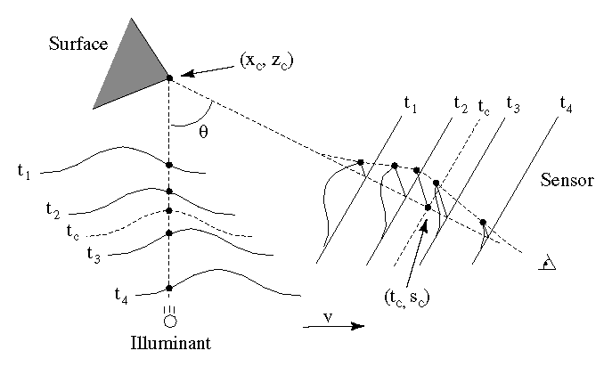
Figure 5: Spacetime mapping of a Gaussian
illuminant. As the light sweeps across the corner point, the
sensor images the shape of the illuminant over time.
For a more rigorous analysis, we consider the time evolution of the
irradiance from a translating differential surface element, ![]() ,
as recorded at the sensor. We refer the reader to
Figure 6 for a description of coordinate systems;
note that in contrast to the previous section, the surface element is
translating instead of the illuminant-sensor assembly.
,
as recorded at the sensor. We refer the reader to
Figure 6 for a description of coordinate systems;
note that in contrast to the previous section, the surface element is
translating instead of the illuminant-sensor assembly.
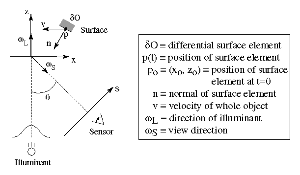
Figure 6: Triangulation scanner coordinate
system. A depiction of the coordinate systems and the vectors
relevant to a moving differential element.
The element has a normal ![]() and an initial position
and an initial position ![]() and is translating with velocity
and is translating with velocity ![]() , so that:
, so that:
![]()
Our objective is to compute the coordinates ![]() given the temporal irradiance variations on the sensor. For
simplicity, we assume that
given the temporal irradiance variations on the sensor. For
simplicity, we assume that ![]() . The illuminant we
consider is a laser with a unidirectional Gaussian radiance profile.
We can describe the total radiance reflected from the element to the
sensor as:
. The illuminant we
consider is a laser with a unidirectional Gaussian radiance profile.
We can describe the total radiance reflected from the element to the
sensor as:
where ![]() is the bidirectional reflection distribution function
(BRDF) of the point
is the bidirectional reflection distribution function
(BRDF) of the point ![]() ,
, ![]() is
the cosine of the angle between the surface and illumination. The
remaining terms describe a point moving in the x-direction under the
Gaussian illuminant of width w and power
is
the cosine of the angle between the surface and illumination. The
remaining terms describe a point moving in the x-direction under the
Gaussian illuminant of width w and power ![]() .
.
Projecting the point ![]() onto the sensor, we find:
onto the sensor, we find:
where s is the position on the sensor and ![]() is the angle
between the sensor and laser directions. We combine
Equations 2-3 to give us an equation
for the irradiance observed at the sensor as a function of time and
position on the sensor:
is the angle
between the sensor and laser directions. We combine
Equations 2-3 to give us an equation
for the irradiance observed at the sensor as a function of time and
position on the sensor:
To simplify this expression, we condense the light reflection terms into one measure:
![]()
which we will refer to as the reflectance coefficient of point
![]() for the given illumination and viewing directions. We also
note that x=vt is a measure of the relative x-displacement of the
point during a scan, and
for the given illumination and viewing directions. We also
note that x=vt is a measure of the relative x-displacement of the
point during a scan, and ![]() is the relation between
sensor coordinates and depth values along the center of the
illuminant. Making these substitutions we have:
is the relation between
sensor coordinates and depth values along the center of the
illuminant. Making these substitutions we have:
This equation describes a Gaussian running along a tilted line
through the spacetime sensor plane or ``spacetime image''. We define
the ``spacetime image'' to be the image whose columns are filled with
sensor scanlines that evolve over time. Through the substitutions
above, position within a column of this image represents displacement
in depth, and position within a row represents time or displacement in
lateral position. Figure 7 shows the theoretical
spacetime image of a single point based on the derivation above, while
Figures 8a and
8b shows the spacetime image generated
during a real scan. From Figure 7, we see that
the tilt angle is ![]() with respect to the z-axis, and the
width of the Gaussian along the line is:
with respect to the z-axis, and the
width of the Gaussian along the line is:
![]()
The peak value of the Gaussian is ![]() , and its mean along the
line is located at
, and its mean along the
line is located at ![]() , the exact location of the range
point. Note that the angle of the line and the width of the Gaussian
are solely determined by the fixed parameters of the scanner,
not the position, orientation, or BRDF of the surface element.
, the exact location of the range
point. Note that the angle of the line and the width of the Gaussian
are solely determined by the fixed parameters of the scanner,
not the position, orientation, or BRDF of the surface element.
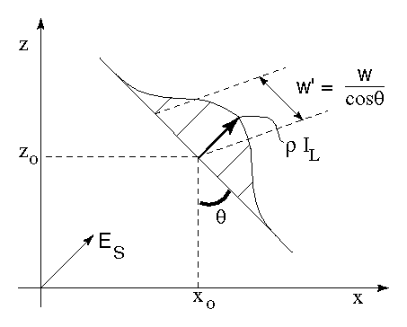
Figure 7: Spacetime image of
a point passing through a Gaussian illuminant.
Thus, extraction of range points should proceed by computing low order statistics along tilted lines through the sensor spacetime image, rather than along columns (scanlines) as in the conventional method. As a result, we can determine the position of the surface element independently of the orientation and BRDF of the element and independently of any other nearby surface elements. In theory, the decoupling of range determination from local shape and reflectance is complete. In practice, optical systems and sensors have filtering and sampling properties that limit the ability to resolve neighboring points. In Figure 8d, for instance, the extracted edges extend slightly beyond their actual bounds. We attribute this artifact to filtering which blurs the exact cutoffs of the edges into neighboring pixels in the spacetime image, causing us to find additional range values.
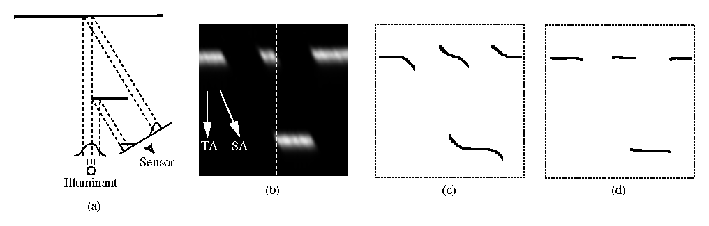
Figure 8: From geometry to spacetime image to range data. (a) The original
geometry. (b) The resulting spacetime image. TA indicates the
direction of traditional analysis, while SA is the direction of the
spacetime analysis. The dotted line corresponds to the scanline
generated at the instant shown in (a). (c) Range data after
traditional mean analysis. (d) Range data after spacetime analysis.
As a side effect of the spacetime analysis, the peak of the Gaussian yields the irradiance at the sensor due to the point. Thus, we automatically obtain an intensity image precisely registered to the range image.
We can easily generalize the previous results to other scanner geometries under the following conditions:
We can weaken each of these restrictions if ![]() does not vary
appreciably for each point as it passes through the illuminant. A
perspective sensor is suitable if the changes in viewing directions
are relatively small for neighboring points inside the illuminant.
This assumption of ``local orthography'' has yielded excellent results
in practice. In addition, we can tolerate a rotational component to
the motion as long as the radius of curvature of the point path is
large relative to the beam width, again minimizing the effects on
does not vary
appreciably for each point as it passes through the illuminant. A
perspective sensor is suitable if the changes in viewing directions
are relatively small for neighboring points inside the illuminant.
This assumption of ``local orthography'' has yielded excellent results
in practice. In addition, we can tolerate a rotational component to
the motion as long as the radius of curvature of the point path is
large relative to the beam width, again minimizing the effects on
![]() .
.
The discussion in sections 3.1-3.3 show how we can go about extracting accurate range data in the presence of shape and reflectance variations, as well as occlusions. But what about laser speckle? Empirical observation of the time evolution of the speckle pattern with our optical triangulation scanner strongly suggests that the image of laser speckle moves as the surface moves. The streaks in the spacetime image of Figure 8b correspond to speckle noise, for the object has uniform reflectance and should result in a spacetime image with uniform peak amplitudes. These streaks are tilted precisely along the direction of the spacetime analysis, indicating that the speckle noise adheres to the surface of the object and behaves as a noisy reflectance variation. Other researchers have observed a ``stationary speckle'' phenomenon as well [1]. Proper analysis of this problem is an open question, likely to be resolved with the study of the governing equations of scalar diffraction theory for imaging of a rough translating surface under coherent Gaussian beam illumination [6].