• KurtBerglund
• Assignment3

You are not allowed to edit this page.

Assignment 3 Camera Simulation

Kurt Berglund

Date submitted: 9 May 2006

Code emailed: 9 May 2006

Compound Lens Simulator

Description of implementation approach and comments

To represent the camera's lens stack, I created a new Lens class for each lens within the stack. A lens simply stores a reference to a pbrt shape primitive which represents the geometry of the lens, as well as some other basic information relating to the lens (indices of refraction, radius). A sphere with its bounds clipped is used for the actual lenses, while a disk with a diameter equal to the passed in camera's aperture size is used to represent the camera's aperture. To find an outgoing ray then, the incoming ray is traced through the stack of lenses. When an intersection occurs, the refracted ray is computed using the Heckbert and Hanrahan method, and the process continues until either the ray exits the camera, or it no longer intersects with a lens, or total internal reflection occurs.

To compute the ray to trace through the lens stack I first map the sample's imageX and imageY positions to a point on the film plane. Then I pass lensU and lensV to ConcentricSampleDisk to compute a point on a disk which is subsequently scaled by the radius of the back lens. The z value for this point on the disk is then set to the z location of the back lens. The origin of the ray is then the film location, and the direction of the ray is the normalized vector from the point on the film plane to the point sampled on the disk which has the same radius and z coordinate as the back lens. In the case that the ray exits the camera, the weight is equal to (area of the disk being sampled) * (cosine between the ray direction and the positive z axis (since this points towards the lens))⁴ / (distance from the back lens to the film)². This weighting follows from the integral described in the paper and the sampling method being used. In the case that the ray does not exit the camera, the weight value returned is 0.

One other issue I ran in to was with with the alpha variable in pbrt's scene render method. As I found while debugging, in the case of a 0 weight ray returned by the camera, this value is uninitalized and is subsequently used by pbrt. In the end, I ended up initializing its value to 1, since in the case of the camera, a ray weight of 0 is a ray which hit the inside of the lens, and so should be treated as a black ray.

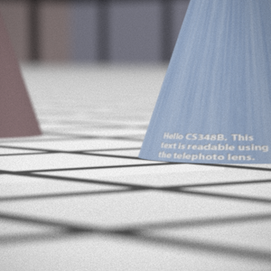
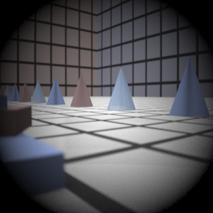
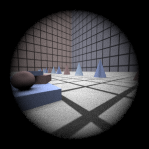
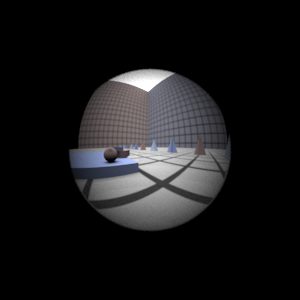
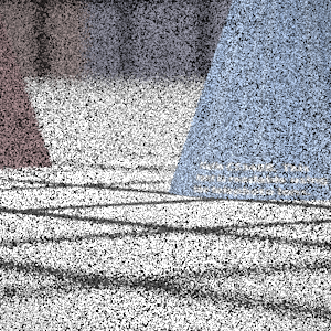
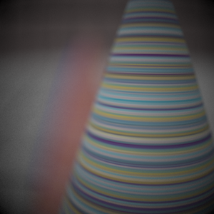
Final Images Rendered with 512 samples per pixel

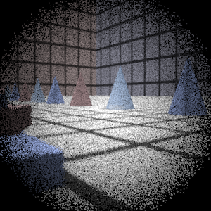
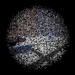
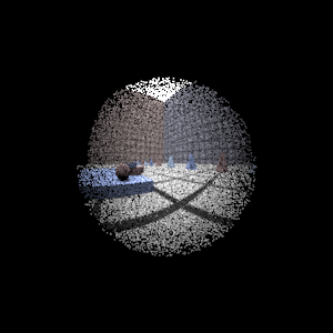
Final Images Rendered with 4 samples per pixel

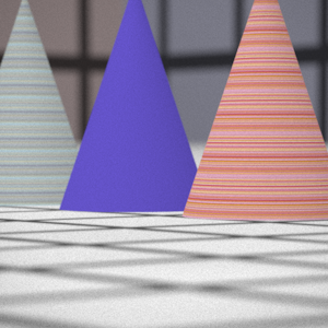
Experiment with Exposure

Observation and Explanation

Reducing the aperture radius in half should have the effect of reducing the exposure by a factor of four (since E = L * PI / 4 * (a/f)²), which causes less light to reach the film and should decrease the brightness by 4 as well, which my camera simulation appears to produce. Because the F-number is the ratio of the focal length divided by the aperture, cutting the aperture in half causes us to double the F-number. Since an Fstop occurs every multiple of sqrt(2), then doubling the F-number causes us to move two Fstops. Thus we've reduced the photograph exposure by two stops, which amounts to halving the exposure twice.

Autofocus Simulation

Description of implementation approach and comments

First, to help with the bounds within which I search for the best film plane depth, I first computed the thick lens approximation to my given lens. I did this the same way as was described in the paper. I had to modify my lens tracing code to be able to go from a ray entering the camera to one leaving its back lens. After this, I shot a ray parallel to the z axis in to the camera and then computed where it intersected the z axis after it exited. This became Fprime. Then, I computed the intersection of this ray with the ray entering the camera, which became Pprime. From this I could then calculate the camera's effective focal length. I did the same thing in the opposite direction as well, but this result wasn't used in my final simulation.

With this value then, to autofocus, I start at the thick lens approximation's focal point, and move down the -z axis away from the lens, incrementing along the way. I used a step size of 2mm and capped the max distance I would move at 100mm, since this worked in practice and seemed like a distance at which I would go past a physical camera's dimensions. Then at each increment I compute the sum modified Laplacian (SML) with a step size of 1 about the entire auto focus region. I initially experimented with the Y value of the XYZ pixel values as the value used in the calculation, since it closely corresponds to perceived brightness, but I didn't find the results to be very good. In the end I used the common (r + g + b) / 3 metric which gave good results.

From watching the output of the SML calculation along the sample space, I saw that there usually is a spike in the SML values when the optimal focus is reached, and then the values quickly drop afterwards. I experimented with heuristics and found that a good exit termination was when the best SML value computed was better than 5/3 * mean value of all computed SMLs, then the depth at the best value was the focal depth to use. I also had tried watching the values and stopping after n values less than the maximum seen, but certain configurations could trick this heuristic. In the end the above seemed to work well.

After computing the above value, I then recursively refine the estimate around the current best guess, using a smaller step size at each refinement, bounded by the step size within which it was computed (i.e. if the best depth is x and my step size was 2mm, my new window is (x - 2) to (x + 2). The recursion stops either when the variance of the computed estimates is < 1 (meaning there isn't much variation, so the image is most likely within focus over that range), or when some max depth is reached (set at 3 in this case). The algorithm can thus be tweaked for speed or accuracy.

I also experimented with the extra autofocus scenes. Whenever there is more than one autofocus zone, my algorithm computes the optimial film depth for each zone independently. Then these depths are sorted, and the distance from each depth to every other is computed. The chosen depth then becomes the value with the smallest summed distance from every other depth. This heuristic made sense to me since it attempts to take the depth value that is as close as possible to the others, hopefully in the process getting a good balance of focus within the scene.

Final Images Rendered with 512 samples per pixel

Any Extras

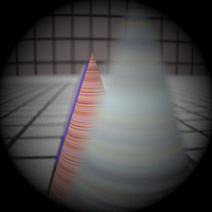
Here are the results of my autofocus algorithm on the harder test cases, using 128 samples per pixel.

The bunny scene was rendered at a film distance of 39.9679 and the other scene was done at 38.3676. With the algorithm I created, the autofocus works as expected. In the second scene, it focuses on one of the objects - since there are only two things, it simply is going to pick one of the two. And in the first scene it puts the focus around the front most bunny. Since the majority of the view sensors fall on objects near it, it is then going to choose one of them to give focus. (Note: There are some visual artificats in this image, but the one on the assignment website had some as well. After doing some investigating, I think the issue had to do with sampling the area light source, since moving the light could remove the artifacts.)