Rendering Multi-Layered Translucent Materials: Overview
For my project I wanted to investigate how to render subsurface scattering from multi-layered translucent surfaces, and did so in the context of trying to render a realistic leaf. As I learned before starting the project, leaves are difficult to correctly simulate, and I certainly found this out from first hand experience. Although I wished I could have had a better looking leaf in the end, I certainly learned a great deal about subsurface scattering, light transport, leaves and BSSRDFs from this project.
Adding the BSSRDF to PBRT
Because the Donner and Jensen paper, which was the method I was planning to use to simulate subsurface scattering, required evaluating a BSSRDF to account for the multiple scattering, the first task I took was to add support for the BSSRDF in to pbrt. As is stated in the major projects section of the book, pbrt has deep seated assumptions that the BSDF is the abstraction used to model surface reflection. Adding BSSRDF support then became a fairly involved project. I did this by adding a new BSSRDF abstract class to the core library, and then for simplicity, added a method to the material class to specify whether the material is using a BSDF or a BSSRDF, as well as methods to return the associated reflection function.
In order to be able to integrate the BSSRDF, it was first necessary to extend the shape class to be able to sample points on the surface of the intersected object. I did this by adding a new GetPoint method to the shape and primitive classes, which would return a point on the surface of the object as well as the pdf for that point. Because I knew that I would be rendering triangle meshes in the end, I only fully implemented this functionality within the triangle mesh plugin. This turned out to be a somewhat complex task. I tried to think of various ways to sample a given triangle mesh. For simplicity and ease of implementation I initially started by only sampling based on the given triangle, which although not correct, still gave fairly good results, but resulted in noticeable edges within the triangle mesh. I then moved on to a method that came up when talking with Professor Hanrahan, that of sampling based on a direction and distance about a given point.
To implement this, I first needed to extend the triangle mesh class to store connectivity information among the edges of the mesh. This allowed me to walk the mesh. Then, based on a given starting point, as well as a direction and distance to travel, my code begins by computing the intersection of the previous ray with the three planes specified by the edges of the triangle and the triangle normal. Then based on the closest intersection, either the algorithm terminates if the distance to the edge is farther than the distance left to travel, or it moves to the intersection point on the edge, updates distance information, and projects the direction vector on to the next triangle (the one that shares that edge). The edge to triangle data structure provides efficient look ups of the triangles attached to a given edge. Once the point in the given direction and distance was found, a DifferentialGeometry structure is created for that point. With this code I was then able to walk a mesh, which made it possible to integrate the BSSRDF.
With the ability to sample a point, I then created a new integrator that was able to integrate a BSSRDF. This integrator was a takeoff on the direct lighting integrator, but with a few modifications. When evaluating a BSDF, the direct lighting integration method is used, otherwise the new BSSRDF integration method is used. This works by first sampling a point about the intersection point on the intersected surface. Then, a sample is taken from a given light source. The lighting is then calculated based on these values, and the resulting PDFs from both sampling the surface and the light source are used to provide the correct Monte Carlo estimator value.
To test these values, I then implemented a new material class based on the Jensen, Marschner, et. Al. paper. I used this mainly to test my mesh sampling methods, and to make sure I had extended pbrt enough, and did not explore this method much more, since I was moving towards the Donner and Jensen method.
Creating a Plant Model
As discussed in Hemenger, leaves are typically a few tenths of a millimeter thick with a layer of tightly fitting cells on each side(epidermis). The interior is then composed of two parts that are of a similar size. The top layer, the palisade layer, consists of elongated parenchyma cells that are regularly arranged perpendicular to the leaf surface, and contains most of the absorbing pigments. The lower layer, called the spongy layer, consists of irregularly arranged parenchyma cells, separated by air spaces that are roughly the size of the cells. Based on this structure, a standard method in the biology literature to simulate a leaf is to break it down in to two layers. Hemenger recommends representing the upper layer as being an absorbing layer and the lower layer as a scattering layer. This causes an enhanced absorption, since the lower layer will scatter light back in to the upper layer, which will be further absorbed.
Due to this representation, I traced the outline of a leaf using NURBS surfaces in 3DS Max to represent a leaf. Then when rendering, I treat this surface as really being composed of two layers, with absorption, scattering, depth, and mean cosine parameters passed as paramters for each layer.
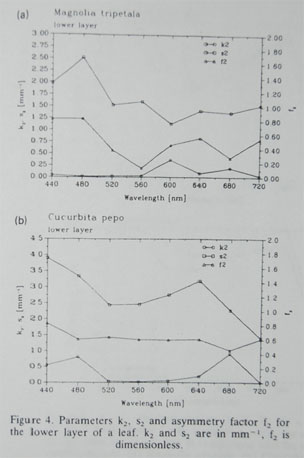
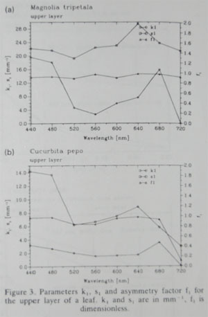
Following the references of the Fukshanksky paper referenced by Donner and Jensen led me to a paper by Martinez et. al. which gave scattering and absorption parameters for the two layers of two types of plant leaves. I was fairly excited after I found these numbers, since I was hoping to accurately simulate a real type of plant leaf based on physically correct parameters. However, in practice, I had difficulty using these numbers with the multi-layer diffusion equation, and ended up using a model presented in the Donner paper with numbers chosen by trial and error. The numbers from the Martinez paper are given at the end in case someone finds them useful in the future.
Rendering the Light Scattering
To render the plant leaves I used three techniques to attempt to simulate the look of the leaf: Monte Carlo integration of the single scattered light, a multi-layer diffusion equation for multiply scattered light, and bump mapping.
Single Scattering
Because the diffusion approximation explained below represents light that has scattered more than one time, I also evaluate the contribution of light that has undergone a single scattering event. I do so by Monte Carlo integrating along the refracted outgoing ray’s path through all layers of the material, as explained in Jensen, et. Al. The surface normal and outgoing/incoming ray directions determines which side of the surface the ray is entering and leaving, and depending on this, I apply the parameters for the appropriate layer the ray is traveling through.
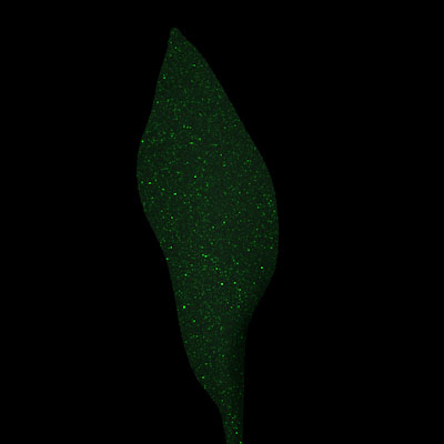
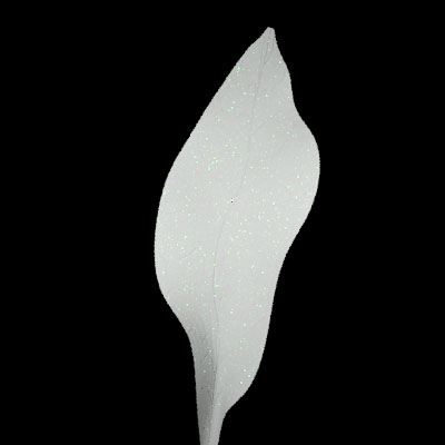
Rendering using the leaf parameters from the Martinez paper results in the following images. Martinez does not give g, the mean cosine of scattering, but rather uses a term f, which is the fraction of forward scattering. I simply use a large g value to represent a larger f value, since the larger g is, the more forward scattering there is. The first image has the light behind the leaf, the other in front. Leaves are highly forward scattering of light, which is why the first image is much brighter than the second.


Multiple Scattering Using the Diffusion Approximation
To account for the light that scatters multiple time, I implemented the method described in the Donner and Jensen paper to calculate light diffusion in multi-layered translucent materials. This turned out to be much more difficult than I had envisioned, as will be explained below.
The diffusion approximation for thin slabs works very similarly to the case of a semi-infinite material. An initial dipole pair is set up over the top surface to maintain the boundary condition that any light leaving the thin-slab does not return. However, because the material is a thin slab, some light may now escape from the slab, rather than just being absorbed or reflected to the top, as was the case for a semi-infinite medium. To account for this a similar boundary condition is set up at the bottom of the slab, with the condition being that any light transmitted through the slab does not return. Another dipole pair is used to maintain the boundary condition at the lower layer. However, adding this dipole pair causes the top boundary condition to no longer hold, and so another dipole pair is used, which in turn violates the bottom condition, etc… An infinite number of pairs are then created, however, since each contributes less and less to the final value, eventually the computation is terminated when the addition of more poles becomes insignificant to the final answer.
In this way I then compute the reflectance and transmittance of each layer based upon the above calculation. I eventually decided upon representing a leaf based on the model described by Donner (a thick absorbing layer over a thin highly scattering layer) which is based on Hemenger’s analysis. Tweaking parameters around this general theme (thick absorbing, thin highly scattering), gave me good reflectance and transmittance values for each slab.
After this I moved on to calculating the diffusion in multi-layered materials due to multiple scattering. This is done by a Fourier transform to the frequency domain. As Donner describes, the transmittance profile for two layers can be computed by convolving the transmission from each layer together. However, this just accounts for light that transmits twice. Light could also have reflected off both layers before transmitting, or reflected multiple times before transmitting. This results in an infinite number of summed convolutions. Converting to the frequency domain though allows us to represent this as a geometric series, since now we are multiplying the various profiles. The combined transmission is then given as TC = T1 * T2 / (1 – R2 * R1) and RC = R1 + T1 * R2 * T1 / (1 – R2 * R1). So long as R2 * R1 < 1, then these equations hold.
This seemed like a fairly simple computation to make, however, it proved to give me a lot of problems. Initially I used a fast fourier transform function from http://astronomy.swin.edu.au/~pbourke/other/fft2d/, however, in the end I ended up doing my computations in Matlab, and then loading in the results. The convolution theorem did not seem to be holding in all cases in Matlab, since a multiplication in the frequency domain did not result in the same output as a convolution in the spatial domain. However, I eventually stumbled upon the Matlab documentation stating that to make this precise, it was necessary to pad the two vectors with zeros, which after I did caused things to work.
The other issue I ran in to was that the product of R2 and R1 was not always < 1. This was because although the integral of the computed BSSRDF profiles were less than 1, they still many times had large spikes in the middle. This caused R2 * R1 to sometimes result in values greater than 1. To get R2 * R1 to be less than 1, I ended up multiplying the reflection and transmission profiles by 0.001, which was the step size the values were computed at, and then performing the operations, before then dividing the result by 0.001 to get the final values. In my mind this was a coordinate change that seemed to take in to account the differential in the integral. I’m not sure if it was the correct thing to do, but it allowed me to apply the formula in the paper, and generally resulted in an output that looked right, so I went with it.
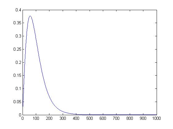
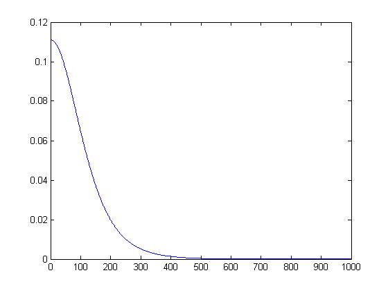
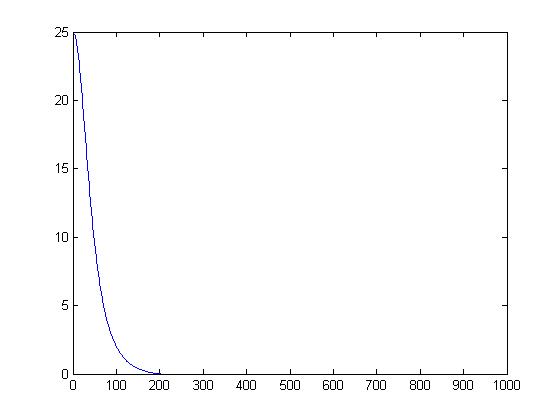
At first I tabulated the reflection and transmission values on a 2D grid, and then put these in to a 2D FFT. However, I noticed the result was radially symmetric, and I ended up turning to just calculating a 1D function based on the radius, and then performing the above stated computations on these. This sped up and simplified computations, and I believe still results in the same output. Another simplification I made due to the padding was to compute the above values on a function of only positive radius’s. This caused everything to look like half a Gaussian curve starting at the origin. Although this doesn’t result in the entirely correct convolutions, it made it easier to sample the function later, and also made it simpler to know where the origin was, since sometimes the output, due to the padding, would make it difficult to find this in the case that both negative and positive values of r were represented in the function. At the end of this report there are graphs showing the original and combined reflectance and transmittance profile created using this method.
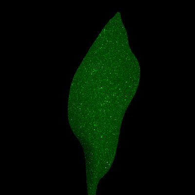
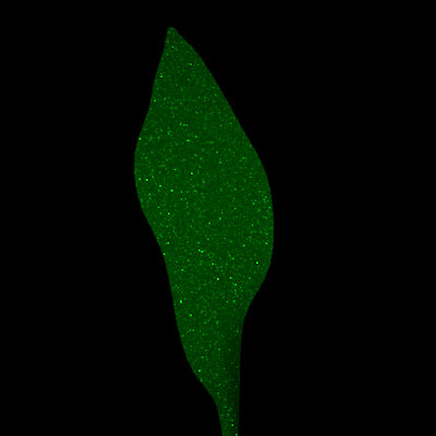
In sum, the reflectance and transmittance values are stored in a table based on the radius, which are then looked up based on the BSSRDF input parameters. I also don’t have much experience with Fourier transforms outside of the basics we learned in class, so dealing with them in this assignment ended up being quite a challenge. Some of my above stated relaxations were probably not the technically correct thing to do, but in the end I was just trying to get transmission and response graphs that seemed right, and so made any changes to get closer to the goal of getting something that looked like a leaf. This process seemed to work, since the following images demonstrate a visual property of leaves - bicoloration. That is, although the reflectance of a leaf may be different depending on orientation, the transmittance is largely the same:
Leaf Front and Back, front lit:
Leaf Front and Back, back lit:
Bump Mapping
I also added bump mapping support to my material so that I could simulate the veins and structure of the leaf. This turned out to be a little harder than I initially imagined, the reason being the wavefront file format plug-in for pbrt. If UV coordinates exist, the plug-in, to simplify implementation, will then duplicate vertices, rather than indexing the same ones each time they appear. My mesh walking code to evaluate the BSSRDF relies on meshes indexing the same vertices to compute edge sharing, so this caused it to believe each triangle was not connected to any others. I had to modify the plug-in code to reference the same vertices and to give the correct UV coordinates in order to to get bump mapping to work. This project was the first time I used a 3D modeling program, so applying the bump map was largely drawing on a texture in Photoshop and then checking if I made the right thing by rendering it in pbrt. If I had more time, I would have learned how to map a texture on to a surface so that I would have had more control over the overall look.
Final Image
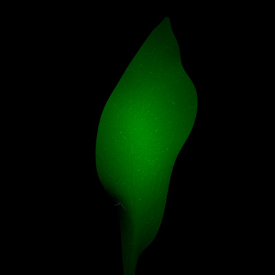
Combining the above three techniques, as well as my leaf model, resulted in the following images (with the light being behind the leaf). The first one was created using the same parameters as were used above to show the bicoloration, and the other was the image shown at the rendering competition. I caught a slight bug while doing this writeup, and so the left image is the result of some parameter tweaks and the bug fix.

Conclusions
As I found while doing this project, simulating a plant leaf is a difficult process. Before the project began, my initial goal was to implement the Donner and Jensen paper, since they provided some very good looking leaves in the paper, and then to extend upon these. However, the subsurface scattering paper was very technically challenging, and was difficult to implement. I spent a good deal of time in the beginning trying to understand the diffusion equation derivation (checking out the Ishimaru book Wave Propagation and Scattering in Random Media) and how it is used in the Donner paper, as well as reading the biology literature, especially to find physically correct scattering and absorption parameters. The technical difficulty of the paper also caused me a lot of difficulty to get it working. The time I invested to learn about the derivation of the method made me really push to try to implement it, even though in terms of creating a more compelling scene, the smarter choice may have been to abandon it and stick with the single scattering. However, I certainly learned a great deal in this project, from more advanced light transport theory, the biology of leaves, taking Fourier and inverse Fourier transforms, adding a BSSRDF to a rendering system, as well as rendering subsurface scattering.
Future Work
There are a lot of things I would try if I ever try render leafs again. For starters, I would attempt to model the internal structure of a leaf (both epidermal layers, as well as the internal layers) with geometric models. This method is used by some biologists to perform Monte Carlo evaluation of the properties of a leaf (see Ustin, et. Al). I would like to either try to estimate a BSDF based upon the structure, or use Monte Carlo integration myself to render the structure based upon the geometry, and see how this compares to the multi-layer estimates.
Another area would be to actually simulate the veins within a leaf. In my research I found SIGGRAPH papers on doing just this. From looking at real leaves, many leaves appear to be multiple “patches” of material, separated by the vein structure. I think due to this structure the multi-layer assumptions may also not be the most correct, and that a more accurate leaf could be made by creating an object of these veins, with patches of the cell structure in between. Then simulating the patches with the geometric structure described above could possibly lead to some very compelling images.
Works Cited
Craig Donner and Henrik Wann Jensen, Light Diffusion in Multi-Layered Translucent Materials
Henrik Wann Jensen, Stephen R. Marschner, Marc Levoy, and Pat Hanrhahan, A Practical Model for Subsurface Light Transport
Alexander Martinez v. Remisowsky, John H. McClendon and Leonid Fukshansky, Estimation of the Optical Parameters and Light Gradients in Leaves: Multi-Flux versus Two-Flux Treatment
R. P. Hemenger, Optical Properties of Turbid Media with Specularly Reflecting Boundaries: Applications to Biological Problems
S. L. Ustin, S. Jacquemoud and Y. Govaerts, Simulation of Photon Transport in a Three-Dimensional Leaf: Implications for Photosynthesis.
Works Referenced
L. Fukshanksy, A. Martinez v. Remisowsky, J. McClendon, A. Ritterbusch, T. Richter and H. Mohr, Absorption spectra of leaves corrected for scattering and distributional error: a radiative transfer and absorption statistics treatment
Pat Hanrahan and Wolfgang Krueger, Reflection from Layered Surfaces due to Subsurface Scattering
Lifeng Wang, Wenle Wang, Julie Dorsey, Xu Yang, Baining Guo and Heung-Yeung Shum, Real-Time Rendering of Plant Leaves
Henrik Wann Jensen and Juan Buhler, A Rapid Hierarchical Rendering Technique for Translucent Materials
Leaf Material Properties from Martinez
Reflectance values (R1, R2)
Transmission values (T1, T2)
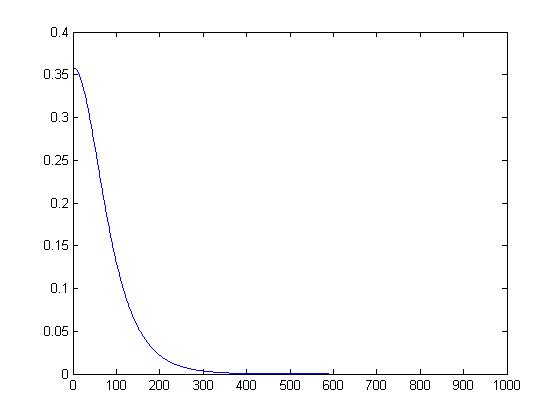
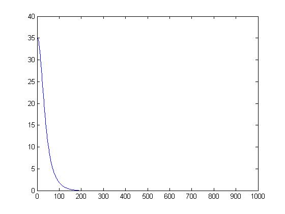
Combined Refelectance, Transmission

