Differences between revisions 2 and 3
| Deletions are marked like this. | Additions are marked like this. |
| Line 4: | Line 4: |
|
== Date submitted: 05 May 2006 == == Code emailed: 05 May 2006 == |
== Date submitted: 08 May 2006 == == Code emailed: 08 May 2006 == |
Assignment 3 Camera Simulation
LeeHendrickson
Date submitted: 08 May 2006
Code emailed: 08 May 2006
Compound Lens Simulator
Description of implementation approach and comments
Given the data file for a lens system, the file is parsed and a "LensSurface" object is created for each element in the system. The LensSurface represents both the aperture stop and the lenses themselves so as to be transparent to the camera itself. Thus, a ray is generated by the camera as follows:
- The initial raster-space sample is converted into camera space
A sample is taken on the back lens using ConcentricSampleDisk
- An initial ray is constructed from these two points and started through the lens system
In order, the ray is intersected with each LensSurface. The LensSurface is responsible for performing either a plane (aperture) or sphere (lens) intersection and returning the necessary intersection information.
- If the ray does not intersect the current lens a "dead ray" is returned by the camera.
- If the ray does intersect the lens, a refraction of the ray is performed using Snell's law accounting for total internal reflection) and the new ray continued through the system.
- If the ray makes it through the entire lens system, it is returned from the camera, with a weighting as defined in Kolb's paper: a cos^4 term multiplied by the area of the back aperture and divided by the square of the distance between the film and back aperture.
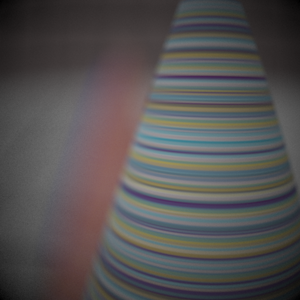
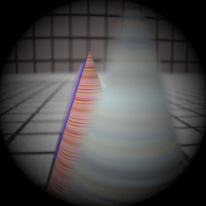
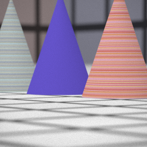
I was lucky in that the tracing system worked without much debugging, the only real problem I encountered was correctly constructing the transformations necessary to convert between camera/raster/lens space. Once these transformations were in place the system produced images closely matching the reference images. Helpful in writing the lens intersection routines was borrowing ideas from pbrt's disk and sphere classes. I also had one lingering bug which was responsible for creating images with a large amount of noise, but this was also eventually squashed.
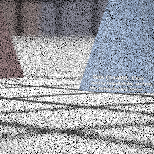
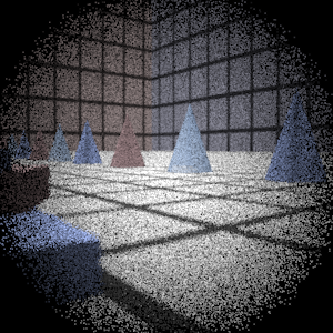
Final Images Rendered with 512 samples per pixel
|
My Implementation |
Reference |
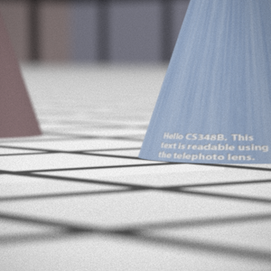
Telephoto |
|
|
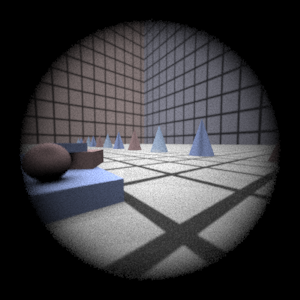
Double Gausss |
|
|
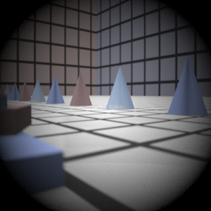
Wide Angle |
|
|
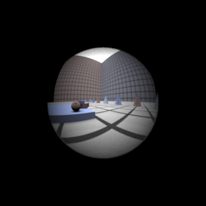
Fisheye |
|
|
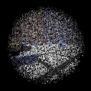
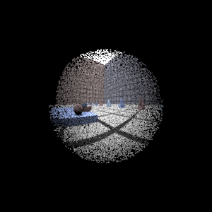
Final Images Rendered with 4 samples per pixel
|
My Implementation |
Reference |
Telephoto |
|
|
Double Gausss |
|
|
Wide Angle |
|
|
Fisheye |
|
|
Experiment with Exposure
Image with aperture full open |
Image with half radius aperture |
|
|
Observation and Explanation
The expectation is that the image will appear darker as a result of the lessened exposure due to the smaller aperture and the camera simulation does produce this result. A reduction of the aperture by one half corresponds roughly to decreasing the photographic exposure by two stops.
Autofocus Simulation
Description of implementation approach and comments
The autofocus algorithm was built using Nayar's concept of a sum-modified Laplacian (SML). For the rgb values generated for an autofocus zone, each value is converted to luminance and the SML calculated for each value using a step size of 1. These SML's are summed over the entire zone to arrive at a scalar focal measure for the current autofocus zone. The maximum focal measure is searched for over a set of autofocus zones each corresponding to a different film distance.
I am not entirely happy with the way this search is actually performed. The focal measures seem to suffer greatly from noise, even taking large amounts of samples (1024 per pixel) in the autofocus sone. The beginning of the range of film distances was simply unusable and the rest of the data was decidedly not unimodal. Thus, the only approach that seemed reasonably robust was an "adaptive" brute-force algorithm. Starting at the far end of the range of film distances, a focal measure is computed at 0.5mm steps moving towards the close end. This "backwards" stepping was to avoid the noisy data at the beginning of the range. Running statistics are kept on each focal measure encountered during the traversal, and when a focal measure is found that deviates greatly from the norm, it is marked. If from that point the focal measures begin to consistently fall then the search is stopped and the film distance corresponding to the marked focal measure is used.
I would like to use a more clever algorithm, such as a bisection of golden-section search but the form of the focal measure data seems to prohibit that approach. The largest drawback to the brute-force approach is that the larger the initial range the longer the algorithm takes to find the correct answer (though it does, eventually), thus its runtime is highly dependent on being fed a reasonable search range at initialization.
Final Images Rendered with 512 samples per pixel
|
Adjusted film distance |
My Implementation |
Reference |
Double Gausss 1 |
62 mm |
|
|
Double Gausss 2 |
39.5 mm |
|
|
Telephoto |
117 mm |
|
|

