Assignment 3 Camera Simulation
Mattias Bergbom
Date submitted: 8 May 2006
Code emailed: 8 May 2006
Compound Lens Simulator
Description of implementation approach and comments
Just as suggested I tried going about this assignment in a slightly more methodical fashion than the previous one. I use a Lens class which holds a std::vector of LensSurface structs, that each describe all properties that are required when tracing rays both from film to world and vice versa. This structure makes it very easy to iterate back and forth through the elements, and by tagging the aperture(s) I can add them into the vector as LensSurfaces as well and treat them transparently. For extra clarity this would probably have been a good place for some genuine OO, but for simplicity I opted for an if statement in the LensSurface::Refract method instead.
Tracing rays through the lens system now boils down to iterating through the LensSurface vector and calling Refract() to do Snell's law on each element, discarding the ray (by returning weight 0) if it goes out of bounds or reflects.
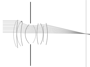
Coming straight out of CS223b, right from the start I decided to use OpenCV's drawing facilities to visualize the rays going through the lens, indicating various events (such as aperture hits, reflections etc.) with different figures (see figure 1). This proved extremely useful during the rest of the assignment, since a lot of the more subtle bugs are way easier to detect visually than by stepping through code and checking numbers. By using preprocessor instructions I was able to completely hide all the visualization code from the release build, to improve performance and avoid build errors on other machines.
|
|
Fig 1a: Visualization of ray tracing through a Gauss lens |
Fig 1b: Tracing parallel incoming rays to determine the thick lens |
One bug that I wasn't able to find by visual means was a faulty Snell's law implementation. It manifested itself as unwanted spherical abberation and a smeared out appearance of the images in general. After advise from the TA I was finally able to pinpoint the problem and switch to Heckbert & Hanrahan's method instead.
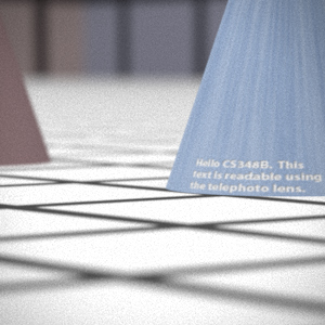
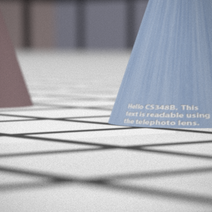
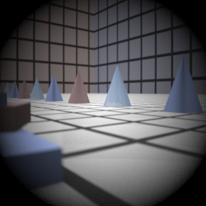
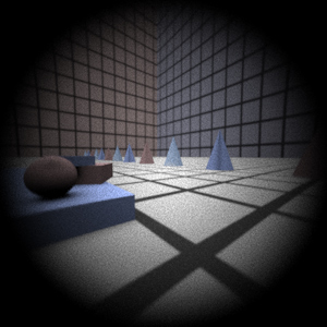
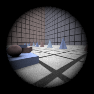
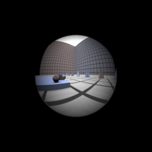
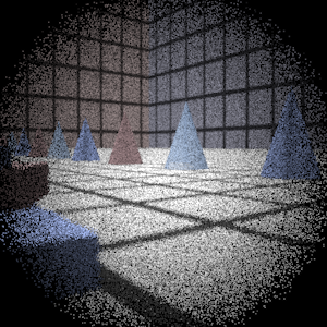
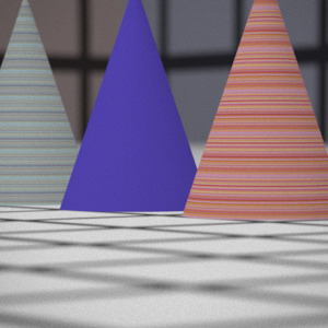
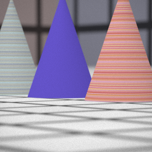
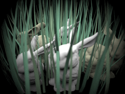
Final Images Rendered with 512 samples per pixel
|
My Implementation |
Reference |
Telephoto |
|
|
Double Gausss |
|
|
Wide Angle |
|
|
Double Gausss |
|
|
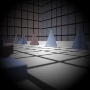
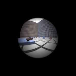
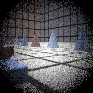
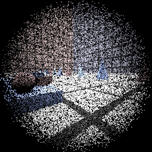
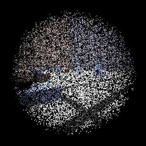
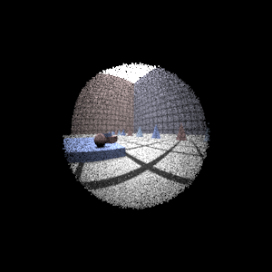
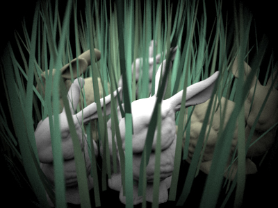
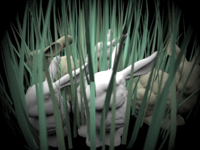
Final Images Rendered with 4 samples per pixel
|
My Implementation |
Reference |
Telephoto |
|
|
Double Gausss |
|
|
Wide Angle |
|
|
Fisheye |
|
|
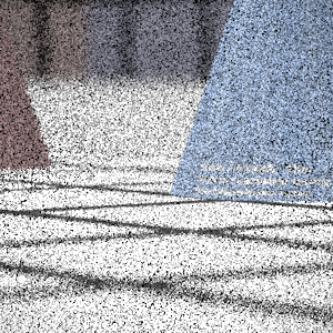
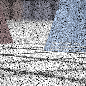
Experiment with Exposure
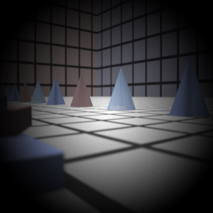
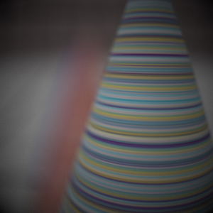
Image with aperture full open |
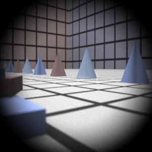
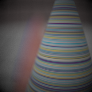
Image with half radius aperture |
|
|
Observation and Explanation
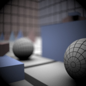
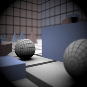
Just as expected, stopping the lens down to half the aperture radius lets less light get in (or 'out'), increasing the exposure and introducing more noise. In this case the exposure time is constant, forcing us to increase the sensitivity of the sensor (i.e. going to higher ASA), which in the classical sense would demand grainier film, and in the modern sense would cause a noisier signal. Also, the depth of field increases as the aperture shrinks, since the peripheral rays that earlier caused wider circles of confusion now are prevented from entering/leaving the lens.
Autofocus Simulation
Description of implementation approach and comments
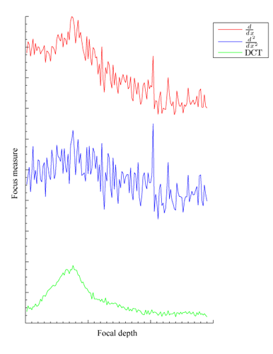
Since derivatives of any order are way too sensitive to the Monte Carlo noise, I quite quickly opted for a DCT (Discrete Cosine Transform) based approach for the 'focusness' measure instead. Any frequency domain method is generally better for noisy data since high frequencies so easily can be filtered out (see Figure 2), and [Kristan 05] presents a very elegant method based on simple 8x8 DCT and Bayes Spectral Entropy. The reasoning behind this approach is in broad strokes that the normalized spectrum of an unfocused image will exibit strong low frequency modes, while a focused image will have its frequencies more uniformly distributed. This property can be captured by using a Bayes entropy function, which is essentially a sum of squares divided by a square of sums:
M(f) = 1 - SUMu v(F(u,v)2)/(SUMu v|F(u,v)|)2
where F(u,v) is the frequency domain function, e.g. the DCT. Kristan also shows that using a regular 8x8 DCT and simply averaging the focus measure over all 8x8 blocks in the focus area is sufficient for robustness, meaning I could go ahead and use any of the abundance of implementations purposed for classic MPEG/JPEG image compression available out there. I settled for a version of the Winograd DCT [Guidon 06]. Also, cutting off some unnecessary frequency content by limiting u+v <= t proved crucial to noise tolerance, and was a key reason that I could step down from the initial 256 samples per pixel to somewhere around 64-128 and maintain robustness.
|
Fig 2: Comparison between DCT-based and derivative-based |
For search, I first did a very naive version that first finds the focal point by shooting parallel rays into the lens and solving for their point of intersection, and starting from there then basically does a number of linear searches with increasing granularity and shrinking search intervals, centered around the maximum in the previous search. Due to the peformance gain of the DCT focus measure method I still land somewhere around 60-100 sec. total with reasonable robustness, which accounts for less than 10% of the total rendering time, but I'm sure there's far more efficient approaches.
|
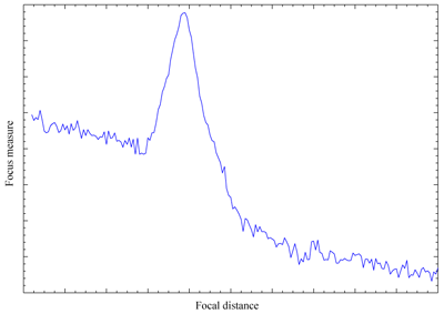
Fig 3: Properties of the BSE method and raytraced images |
One thing that really helped me out during the entire AF ordeal was making lots of plots. By doing high resolution test runs and dumping the results to file, I was able to get an intuitive feel for the problem and quickly find out which approaches to use and which to avoid. For example, although figure 2 suggests unimodality, there's situations where this just doens't hold. I'm not sure if it's related to special properties of ray-traced images in combination with the BSE method, but as figure 3 clearly shows, hw3.dgauss_closeup.pbrt actually seems to decrease in 'focusness' right before the focused plane appears.
This information prompted me to abandon my golden section search at an early stage, and avoid hours of debugging. Furthermore, searching a non-unimodal, noisy function for the global maximum is a problem that as far as I can tell still remains unsolved, at least without significant knowledge of the function's properties. Gaining such knowledge would probably make for an interesting complement to this assignment, one that I unfortunately don't have time for at this point. I'm also interested in what 'statistical' (random) methods one could employ, although I have a hard time seeing they would contribute much in terms of speed due to the amount of samples required.
References:
M. Kristan, J. Pers, M. Perse, S. Kovacic. "Bayes Spectral Entropy-Based Measure of Camera Focus". Faculty of Electrical Engineering, University of Ljubljana. 2005.
Y. Guidon. "8-tap Winograd DCT optimised for FC0". <http://f-cpu.seul.org/whygee/dct_fc0/dct_fc0.html>. 2002.
Final Images Rendered with 512 samples per pixel
|
Adjusted film distance |
My Implementation |
Reference |
Double Gauss 1 |
61.5 mm |
|
|
Double Gauss 2 |
39.6 mm |
|
|
Telephoto |
116.2 mm |
|
|
Extras
Multi-zone AF
Since the focus measure function always is positive, an average of several AF zones will never cause any cancellation or severe damping of peaks. Also, with the very sharp, narrow peaks displayed by the BSE function, artificial peaks in overlap zones aren't very likely, but rather a slight smearing of the solution will take place. Interesting intervals in the focus depth will thus remain significant, and will be found given that the search method is sane.
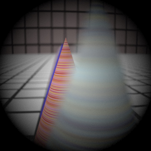
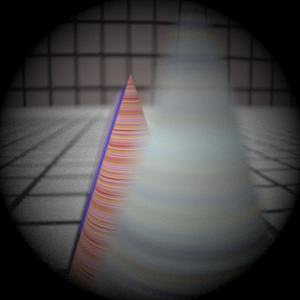
Thus I started off by simply averaging all the zones uniformly to get a focus function, and did a standard search on it. This turned out fairly well (see Figure 4) but I also wanted to try some other approaches. The second one I tried was to search each zone individually, and then, based on some weighting, pick the zone that had the highest peak value. In order to do the weighting, I stored each zone's distance to the center of the image during initialization, and used it in a weighting function, giving priority either to the center (Figure 5a), the periphery or uniformly (which would hopefully correspond to the averaging result).
Due to the content of the image, the center and periphery modes produced pretty similar results though, so I also added weighting towards different directions in the image, which is something any photographer would want when composing. For example top weighted AF (Figure 5b) will simply subtract the zone's fractional y position in the image from 0.5 and use that as a weight, giving zones above the middle of the image increasing priority. I also added a macro mode (Figure 6a-b), where the weighting instead is done using some function of the focal depth. Macro modes usually involve searching a smaller (and closer) interval of the focal measure function as well (for speed and simplicity), but time prohibited me from finding a good heuristic for that.
To try out the different AF modes, add a string variable called "af_mode" to the camera settings, with one of the following values (uniform is default): uniform, center, periphery, macro, left, right, top, bottom. I would be very curious to know how things work out, since I couldn't possibly try out all of the settings. None of this should have any effect if there's one or fewer AF zones.
|
Fig 4: Result of simple averaging of AF zones. |
|
|
Fig 5a: Result of center weighted AF. |
Fig 5b: Result of top weighted AF. |
|
|
Fig 6a: Result of macro AF. |
Fig 6b: Result of uniform AF. |

