Differences between revisions 46 and 47
| Deletions are marked like this. | Additions are marked like this. |
| Line 57: | Line 57: |
| To calculate exactly where this maximum occurs, the program starts by calculating the SML values starting from the focal length distance. The current maximum SML value is stored; if the current SML value is greater than the current maximum SML value, then it tries to notice a decreasing trend following the maximum. If there are 5 montonically decreasing values following this maximum, then the loop is exited and the film distance is set equal to the distance which has the current maximum SML value. This method works because, the focus point is a very defined maximum, with monotonically increasing values leading up to it and then monotonically decreasing values leading away from it; in this manner, it differentiates itself from the noise surrounding it on either side as shown in the graphs. | To calculate exactly where this maximum occurs, the program starts by calculating the SML values starting from the focal length distance. The current maximum SML value is stored; if the current SML value is greater than the current maximum SML value, then it tries to notice a decreasing trend following the maximum. If there are 5 montonically decreasing values following this maximum, then the loop is exited and the film distance is set equal to the distance which has the current maximum SML value. This method works because, the focus point is a very defined maximum, with monotonically increasing values leading up to it and then monotonically decreasing values leading away from it; in this manner, it differentiates itself from the noise surrounding it on either side, as shown in the graphs. |
Assignment 3 Camera Simulation
Name: Ranjitha Kumar
Date submitted: 7 May 2006
Code emailed: 7 May 2006
Compound Lens Simulator
Description of implementation approach and comments
The first part of the assignment was to implement RealisticCamera::GenerateRay. There were two main tasks in the function: first, you had to set up a ray, and then you had to trace that ray through the lens system.
To setup a ray, the program chooses a point on the film plane, the origin of the ray, and a point on a disk with a raidus that is equal to the radius of the aperture of the back lens element, which will determine the direction of the ray. To choose the point on the film plane, which is perpendicular to the z-axis, the program maps the point (sample->imageX, sample->imageY) given in raster coordinates to camera coordinates. Using the film diagonal given in mm, the program determines the film's dimensions in camera space, and centers the film in the xy plane. The z-coordinate of the ray, which is the z coordinate of the film, is determined by adding up all the axpos's of the lens system and the film distance. Next, ConcentricSampleDisk() is used to achieve uniform area sampling on the lens disk corresponding to the back lens element. The point returned by ConcentricSampleDisk is scaled the radius of the back lens aperture. (It is assumed that the lens disk and the film plane are parallel to each other.) Given these two points, a ray is constructed which is directed towards the lens elements.
After having constructed the ray, the ray is traced through the lens system. Tracing consists of two main parts: first a ray sphere intersection is performed (we are assuming spherical lenses), and second, after finding the point of intersection on the lens, Snell's law is used to determine the new direction of the ray after refracting through the lens surface. The ray-sphere intersection is performed by substituting the parametric equation of a ray into sphere equation with a translated z-Center: x2 + y2 + (z-centerZ)2 - r2 = 0. The quadratic equation is solved for t. If there are two solutions, the program chooses the smaller solution if the ray is intersecting with a surface with negative radius, and the larger solution if it is intersecting with a surface with positive radius. On the other hand if the ray is going through the aperture, a ray-plane intersection is calculated. After finding an intersection point, a test is done to determine whether the intersection point is on the lens or inside the aperture opening. The test is the same in both cases: compute the distance from the z-axis and determine whether it is within the aperture radius. If the intersection point is valid, Snell's law is used to determine the direction after refracting with the lens surface. The program implements the vector form of Snell's law derived by Heckbert and Hanrahan: http://www.cs.cmu.edu/~ph/refr.ps.gz. I initially tried computing Snell's law using angles, and it proved to extremely confusing. For the equation presented in the paper, the normal's direction is define to be opposite of that of the incident ray. A normal on a sphere's intersection point is computed as being the vector defined by the center of the sphere minus the intersection point. (The resulting vector might need to be multiplied by -1 depending on the sign of the radius, so that the normal points in the opposite direction of the incoming light ray.)
GenerateRay returns a weight for every ray. I weight my rays by computing (1/(film distance)2)*(Area of the back element of the disk)*(cos(theta))4 as proved in the Kolb paper. If a ray failed to make it through the lens system, it is given 0 weight.
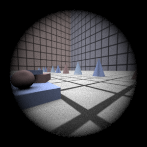
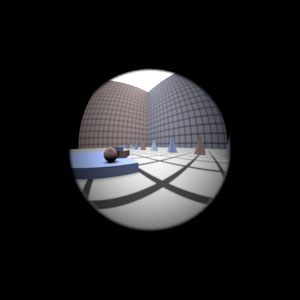
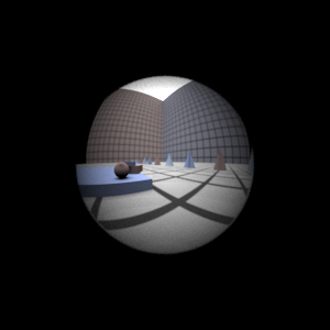
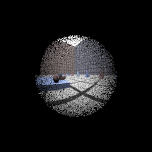
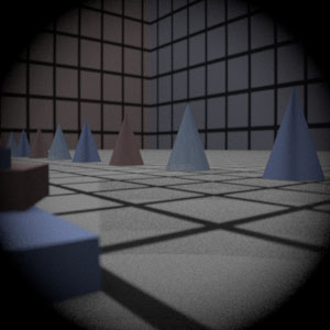
Final Images Rendered with 512 samples per pixel
|
My Implementation |
Reference |
Telephoto |
|
|
Double Gausss |
|
|
Wide Angle |
|
|
Fisheye |
|
|
Final Images Rendered with 4 samples per pixel
|
My Implementation |
Reference |
Telephoto |
|
|
Double Gausss |
|
|
Wide Angle |
|
|
Fisheye |
|
|
Experiment with Exposure
Image with aperture full open |
Image with half radius aperture |
|
|
Observation and Explanation
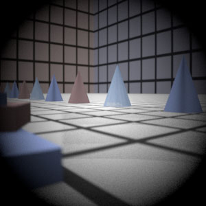
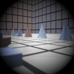
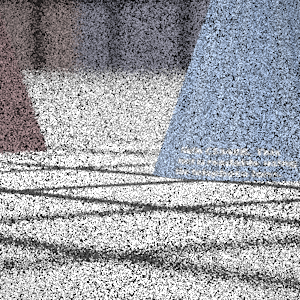
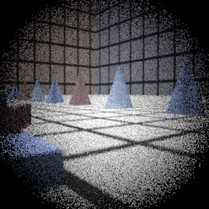
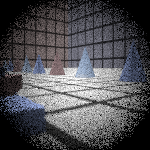
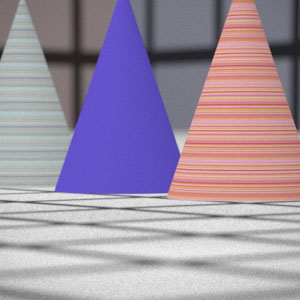
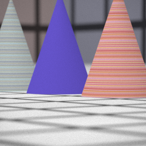
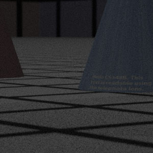
When you reduce the aperture radius by one half and keep the shutter speed the same, you expect that the image will be darker and noisier because fewer rays make it through the lens system and onto the film plane. This effect is illustrated by the images rendered above. Also notice how the foreground in the image on the right appears sharper than that of the image on the left; making the aperture smaller increases the depth of field because the circles of confusion are forced to be smaller; this concept is better illustrated by the stopped down renderings with the telephoto lens (see Extras below.) When you half the aperture size, you have decreased the photograph exposure by 2 stops.
Autofocus Simulation
Description of implementation approach and comments
I use the "Sum-Modified Laplacian" operator described in this paper by Sree Nayar to measure focus in my autofocus zones. The modified laplacian is defined as the sum of the absolute value of the partial second derivatives. So, in its discrete form it is presented as the following:
- ML(x,y) = |2*I(x,y) - I(x-step,y) - I(x+step,y)| + |2*I(x,y) - I(x,y-step) - I(x,y+step)|
(x,y) defines a pixel postion in the auto focus region and I(x,y) represents the radiance value stored in the region. So given the RGB matrix return by CameraSensor::ComputeImageRGB(), I compute the Sum-Modified-Laplacian, which is the summation of the modified laplacian values over all pixels in the region. For every pixel, I computed the ML separately for every color channel (RGB), and the took the square root of the sum of their squares to arrive at the final ML value for that pixel. (I chose step to be 1, since the autofocus regions were only a few pixels in dimension.) So for a given filmdistance, the autofocus region is sampled and computed, and a SML value is computed for that region based on the RGB array that is returned. To determine where to place the film, the program computes where the SML is the greatest within a range of distances; since the Laplacian is a high-pass filter, a large SML value probably corresponds to a region where edges and textures are in focus.
The program searches for this maximum in the range [focalLength, 2*focalLength]. Since rays from infinity get focused at the focal length, there is no point in computing SML values for film distances which are less than the focal length. Furthermore, the scenes do not appear to have any objects right up against the lens, therefore, it is safe to assume that largest desired magnification is 1:1, which occurs at filmDistance = 2*focalLength.
The focal length is calculated by passing a few parallel rays from the object side of the lens to the image side, and then computing where the exiting ray intersects the z-axis.

Just to get a feel for the SML values being calculated, I calculated the SML values from 0 to 100 at 1 mm granularity for the two dgauss scenes that we had to autofocus. The pink line represents the values calculated from the "bg" file and the navy blue line represents the values calculated from the "closeup" file. (These were calculed using 256 total samples.) Notice how past the focal length, which is about 36 mm for this lens, there is clearly one SML maximum. Therefore, the SML is indeed a good measure of focus, since these distances coincide exactly with where the focus images are produced.
To calculate exactly where this maximum occurs, the program starts by calculating the SML values starting from the focal length distance. The current maximum SML value is stored; if the current SML value is greater than the current maximum SML value, then it tries to notice a decreasing trend following the maximum. If there are 5 montonically decreasing values following this maximum, then the loop is exited and the film distance is set equal to the distance which has the current maximum SML value. This method works because, the focus point is a very defined maximum, with monotonically increasing values leading up to it and then monotonically decreasing values leading away from it; in this manner, it differentiates itself from the noise surrounding it on either side, as shown in the graphs.
Final Images Rendered with 512 samples per pixel
|
Adjusted film distance |
My Implementation |
Reference |
Double Gausss 1 |
62 mm |
|
|
Double Gausss 2 |
40 mm |
|
|
Telephoto |
117 mm |
|
|
Extras
Stop Down the Telephoto Lens
Decreased 4 stops |
Decreased 4 stops + exposure 4X in Photoshop |
Full Aperture |
|
|
|
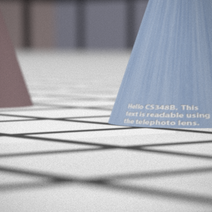
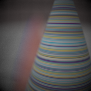
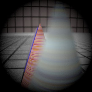
By decreasing the aperture radius to one fourth its original value (4 stops), you can achieve a greater depth of focus. To better illustrate the increase in depth of field I created the rendering in the middle by taking the rendering to the left and changing the exposure to 4 in Photoshop. Notice how the near foreground and background, which appeared fuzzy in the full aperture rendering, now appear sharp and in focus. On an regular camera, if you increased the shutter speed by 16 times, you would get the image in the middle minus the noise.
More Complex Auto Focus
Regular - 39 mm |
Macro-Mode - 42 mm |
|
|
As suggested in the assignment handout, when rendering with multiple autofocus zones, I specify in the scenefile a "string afMode", which has either "macro" or "bg" as input, telling the camera whether to prioritize foreground or background objects. (The afMode is set to "bg" by default.) Then, for each afZone I calculate the distance at which the afZone is the sharpest using the same method as above. If the scene has specified "macro" mode, I set the film distance to be the largest distance out of all the "in focus" distances calculated; if the scene is in "bg" mode, then I set the film distance to be the smallest out all of them. (Closer objects are focused further back, and farther objects are focused closer to the lens.)
The renderings above were made using two autofocus regions. The first autofocus region was sharpest at 39 mm and the second autofocus region was sharpest at 42 mm; so in "bg" mode, the distance given by the first autofocus region was the one that was used, and in "macro" mode, the distance given by the second autofocus region was the one that was used.
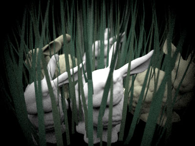
Also, if you have more than one afZone, and a lot of the focus distances are clumped together, you probably want to chose the median value near the front or the median value near the back or even the median of the whole set. I believe my autofocus algorithm didn't fare well given the bunny scene for this reason, which is focused at a midground region. The following are the focused distances returned by the 9 afZones; after sorting them, I rendered the bunny scene at the median distance which is 39 mm, which most closely matched the image given on the assignment page.
- focused distances for the 9 afZones in original order: 60, 39, 39, 39, 37, 40, 50, 39, 40
- sorted: 37, 39, 39, 39, 39, 40, 40, 50, 60
