Assignment 3 Camera Simulation
Name: Ranjitha Kumar
Date submitted: 7 May 2006
Code emailed: 7 May 2006
Compound Lens Simulator
Description of implementation approach and comments
The first part of the assignment was to implement RealisticCamera::GenerateRay. There were two main tasks in the function: first, you had to set up a ray, and then you had to trace that ray through the lens system. To setup a ray, you have to choose a point on the film plane, the origin of the ray, and a point on a disk with a raidus that is equal to the radius of the aperture of the back lens element, which will determine the direction of the ray.
To choose the point on the film plane, which is perpendicular to the z-axis, the program maps the point (sample->imageX, sample->imageY) given in raster coordinates to camera coordinates. Using the film diagonal given in mm, the program determines the dimensions in camera space, and centers the film in the xy plane. The z-coordinate of the ray is determined by adding up all the axpos's of the lens system and the film distance.
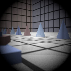
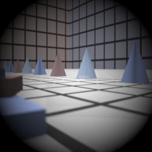
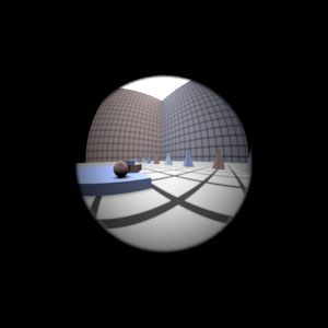
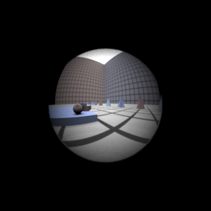
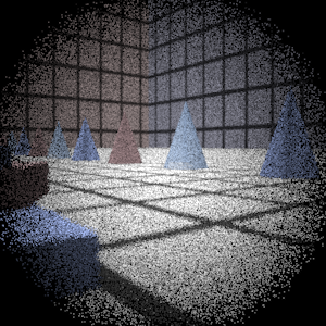
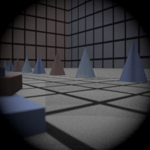
Final Images Rendered with 512 samples per pixel
|
My Implementation |
Reference |
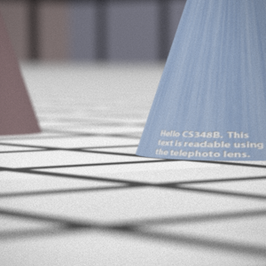
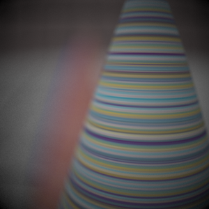
Telephoto |
|
|
Double Gausss |
|
|
Wide Angle |
|
|
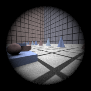
Fisheye |
|
|
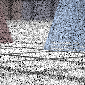
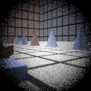
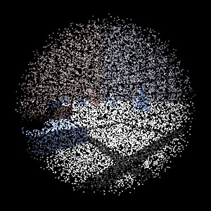
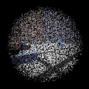
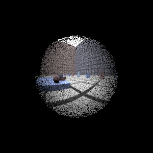
Final Images Rendered with 4 samples per pixel
|
My Implementation |
Reference |
Telephoto |
|
|
Double Gausss |
|
|
Wide Angle |
|
|
Fisheye |
|
|
Experiment with Exposure
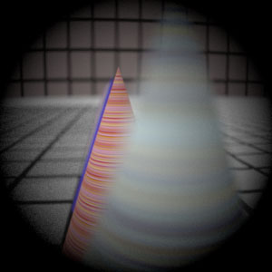
Image with aperture full open |
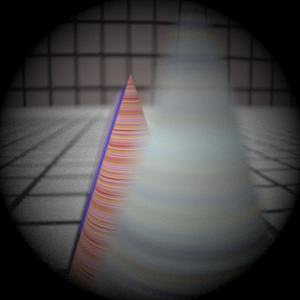
Image with half radius aperture |
|
|
Observation and Explanation
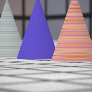
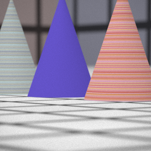
When you reduce the aperture radius by one half and keep the shutter speed the same, you expect that the image will be darker and noisier because fewer rays make it through the lens system and onto the film plane. This effect is illustrated by the images rendered above. Also notice how the foreground in the image on the right appears sharper than that of the image on the left; making the aperture smaller increases the depth of field because the circles of confusion are forced to be smaller; this concept is better illustrated by the stopped down renderings with the telephoto lens (see Extras below.) When you half the aperture size, you have decreased the photograph exposure by 2 stops.
Autofocus Simulation
Description of implementation approach and comments
I use the "Sum-Modified Laplacian" operator described in this paper by Sree Nayar to measure focus in my autofocus zones. The modified laplacian is defined as the sum of the absolute value of the partial second derivatives. So, in its discrete form it is presented as the following:
- ML(x,y) = |2*I(x,y) - I(x-step,y) - I(x+step,y)| + |2*I(x,y) - I(x,y-step) - I(x,y+step)|
(x,y) defines a pixel postion in the auto focus region and I(x,y) represents the radiance value stored in the region. So given the RGB matrix return by CameraSensor::ComputeImageRGB(), I compute the Sum-Modified-Laplacian, which is the summation of the modified laplacian values over all pixels in the region. For every pixel, I computed the ML separately for every color channel (RGB), and the took the square root of the sum of their squares to arrive at the final ML value for that pixel. (I chose step to be 1, since the autofocus regions were only a few pixels in dimension.) So for a given filmdistance, the autofocus region is sampled and computed, and a SML value is computed for that region based on the RGB array that is returned. To determine where to place the film, the program computes where the SML is the greatest within a range of distances; since the Laplacian is a high-pass filter, a large SML value probably corresponds to a region where edges and textures are in focus.
The program searches for this maximum in the range [focalLength, 2*focalLength]. Since rays from infinity get focused at the focal length, there is no point in computing SML values for film distances which are less than the focal length. Furthermore, the scenes do not appear to have any objects right up against the lens, therefore, it is safe to assume that largest desired magnification is 1:1, which occurs at filmDistance = 2*focalLength.
The focal length is calculated by passing a few parallel rays from the object side of the lens to the image side, and then computing where the exiting ray intersects the z-axis.

Final Images Rendered with 512 samples per pixel
|
Adjusted film distance |
My Implementation |
Reference |
Double Gausss 1 |
62 mm |
|
|
Double Gausss 2 |
40 mm |
|
|
Telephoto |
117 mm |
|
|
Extras
Stop Down the Telephoto Lens
Decreased 4 stops |
Decreased 4 stops + exposure 4X in Photoshop |
Full Aperture |
|
|
|
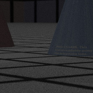
By decreasing the aperture radius to one fourth its original value (4 stops), you can achieve a greater depth of focus. To better illustrate the increase in depth of field I created the rendering in the middle by taking the rendering to the left and changing the exposure to 4 in Photoshop. Notice how the near foreground and background, which appeared fuzzy in the full aperture rendering, now appear sharp and in focus. On an regular camera, if you increased the shutter speed by 16 times, you would get the image in the middle minus the noise.
More Complex Auto Focus
Regular - 39 mm |
Macro-Mode - 42 mm |
|
|
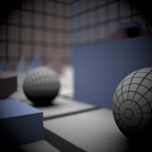
As suggested in the assignment handout, when rendering with multiple autofocus zones, I specify in the scenefile a "string afMode", which has either "macro" or "bg" as input, telling the camera whether to prioritize foreground or background objects. (The afMode is set to "bg" by default.) Then, for each afZone I calculate the distance at which the afZone is the sharpest using the same method as above. If the scene has specified "macro" mode, I set the film distance to be the largest distance out of all the "in focus" distances calculated; if the scene is in "bg" mode, then I set the film distance to be the smallest out all of them. (Closer objects are focused further back, and farther objects are focused closer to the lens.)
The renderings above were made using two autofocus regions. The first autofocus region was sharpest at 39 mm and the second autofocus region was sharpest at 42 mm; so in "bg" mode, the distance given by the first autofocus region was the one that was used, and in "macro" mode, the distance given by the second autofocus region was the one that was used.
Also, if you have more than one afZone, and a lot of the focus distances are clumped together, you probably want to chose the median value near the front or the median value near the back. I believe my autofocus algorithm didn't fare well given the bunny scene for this reason.

