• RyanSmith
• Assignment3

Assignment 3 Camera Simulation

Ryan Smith

Date submitted: 5 May 2006

Code emailed: 5 May 2006

Compound Lens Simulator

Description of implementation approach and comments

My implementation is fairly straightforward. I define a class called Lens Element which is constructed with the parameters from the lens data file. The base Lens Element implementation is a spherical, refracting lens which follows Snell's Law. I use a virtual Intersect method to develop the derived class Aperture Stop, which corresponds to the real aperture stop in a camera. I chose to record both the "left" and "right" indices of refraction in a single Lens Element; this made each element of the lens stack independent, and made the main traversal very concise.

I convert the initial sample position into a film coordinate in camera space; my lens stack grows along the negative Z axis of camera space. Then I use the Concentric Sample Disk function to sample across the back element of the lens system. I generate a ray through these two points in camera space, and send the ray through the lens system. Blocked rays are weighted by 0, and rays that get all the way through the system are weighted with A * cos^{4 over Z}2, where A is the area of the backmost lens element taken as a disk.

I had a brief bit of difficulty with my implentation of ray-disk intersection; this was used for implementing the aperture stop. I had a sign error and was computing an intersection with the aperture plane reflected around Z = 0; this led to a lot of rays getting blocked and the resulting image having a very small visible area.

Other than that, I spent a lot of time trying to figure out why my implementation didn't match the reference images (probably too much time!). However, it wasn't all wasted time, because I tried out several different weighting schemes to try and track down the problem; one method was to cache the first hit position and first hit normal, and really weight the rays by cos(t1) * cos(t2) / mag(dist). The difference was very slight, and in my final implementation i've just used the cos^4 version.

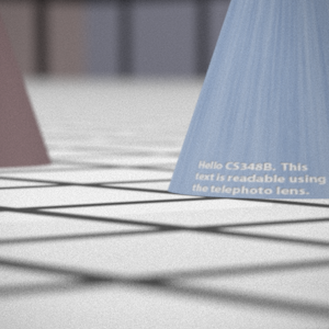
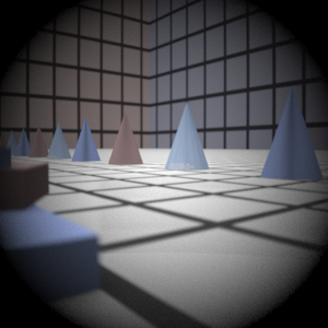
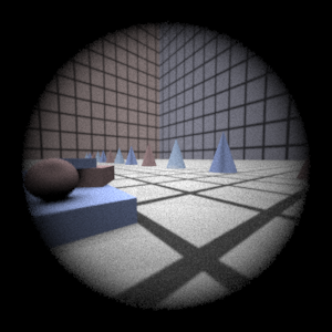
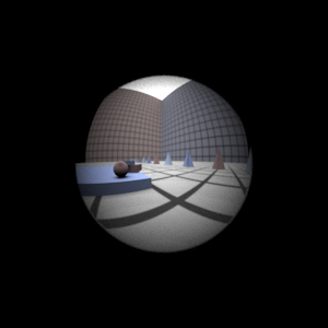
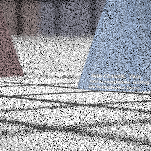
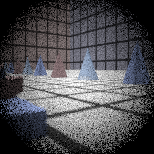
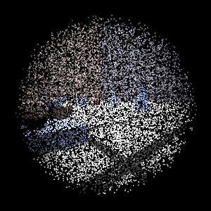
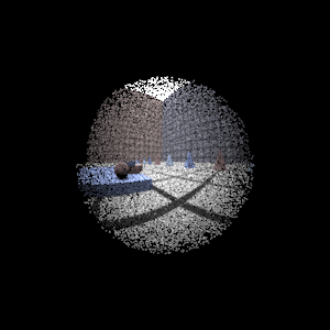
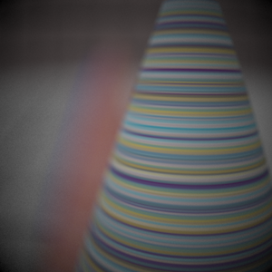
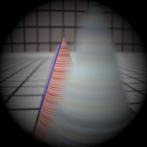
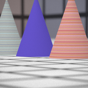
Final Images Rendered with 512 samples per pixel

Final Images Rendered with 4 samples per pixel

Experiment with Exposure

Observation and Explanation

When you reduce the aperture, less light is allowed in, so the picture should be darker. That is what happens in the images from the simulation. The ratio between the areas of the two apertures is approximately 4 (or 1/4, depending), and one stop corresponds to a doubling of area, so we have changed the exposure by approximately 2 stops.

Autofocus Simulation

Description of implementation approach and comments

I used the image based mechanism for autofocus recommended in the assignment. I compute the summed modified Laplacian by first computing the modifed Laplacian for every pixel in the AF zone using I = (R + G + B)/3 and a step size of 1; then I sum the values over the whole autofocus zone.

The main characteristics of the SML results of the images below that drove the design of my algorithm were 1) lots of high SML values when the film displacement was small 2) _very_ high peaks at in-focus positions 3) even aside from the noise at the beginning, the SML of the telephoto image was not unimodal.

To get around the noise at the beginning, I decided to start my search from the far end of the range of reasonable distances. In my final code, the search starts at 200 mm; it could be a lens parameter, and I did vary it in development, but just as an optimization.

I wanted to early out of the search, so that I would stop as soon as I had recognized a peak -- if I kept going until I hit the noise near the back lens element, I would probably eclipse my max focus measure and decide to put the film plane there. However, most of my early out techniques (looking for consecutive decreasing SML values) would get caught up on small bumps in the input data. I took advantage of the fact that I had very high peaks at the in-focus positions by keeping a running average and only acknowledging peaks when the current input value was some ratio (2.0) of the average. Since I had very high peaks (3 - 5x the average) I was able to still catch peaks even though my initial search didn't land right on them.

My linear search operates in two passes. The first pass starts at the far distance and moves towards the back lens element in fixed size, relatively large increments. I record peaks as described above, and stop the search when I have seen some number of consective values less than the last recorded peak. In order to make this stopping condition a bit more robust, I change the film plane increments to a smaller size after I have recorded a peak. This was the only one of my ideas for adaptive sampling that worked.

After the first search executes to completion, I search the range around the highest recorded peak with a finer sampling (0.5 mm) to decide I have the best value.

There are a few shortcomings to this mechanism; the initial search step size could be too large for certain input data, and data without significant peaks might not trigger the "above average" condition. Since the condition was just a mechanism for avoiding the early out, an interesting change would be to search the whole range but to really detect peaks instead of just a "max" value. That is to say, only consider values that were followed by consecutive lesser values as peaks; this would avoid considering the noise at short distances as a peak, since the noise is generally increasing towards the back element. As it is, I don't necessarily have to search the entire range, but certain input might not trigger my peak criteria.

Final Images Rendered with 512 samples per pixel

Any Extras

No extras this time around.